Difference Finite Scheme of Diffusive Equation derived from Lattice Boltzmann
Due to the similarities in the grid structure between the Lattice Boltzmann method and finite difference schemes, several studies have been conducted over the years to investigate how these methods can be directly related and interpreted [3, 4, 5, 6, 7, 8]. In this section, we develop a finite-difference interpretation for different Lattice Boltzmann formulations.
Interpretation for Diffusive Equation
In the remainder of this section, we develop a FDM interpretation of the diffusive LBM, following the approach proposed by Suga [5].
Given the LBM formulation for the diffusive equation:
where the equilibrium distribution function is defined by
and the equilibrium moments are given by
Through Chapman–Enskog analysis, it is demonstrated that the first-order non-equilibrium moment describes the pressure gradient and, consequently, the average velocity:
FDM Interpretation
For simplification we redefine the notation for \(f_i( x_{\alpha} + e_{i,\alpha} \delta t, t+\delta t)=f_{i,x+c_{i}}^{t+1}\). Reinterpreting the Eq. (55) in pre-streaming moment:
Summing the Eq. (58) over all lattice direction and replacing \(f_{i}^{eq}\) by Eq. (56), we have:
using the Eq. (57) to replace \(f_{i,x-c_{i}}^{t}\) in the above equation:
Spliting the terms in the above equation and using Eq. (58) for \(f_{i,x-c_{i}}^{t}\):
doing the same initial procedure to the terms \(f_{k,x-c_{i}}^{t-1}\):
notice that \(\displaystyle\sum_{i}\Bigg( \displaystyle\sum_{k\neq i} \left( \omega w_{k} \phi_{x-c_{i}-c_{k}}^{t-1} \right) \Bigg)=\displaystyle\sum_{i}\Bigg( \displaystyle\sum_{k\neq i} \left(w_{k}\right) \omega \phi_{x+c_{i}}^{t-1} \Bigg)\) and using Eq. (57) we have \(\displaystyle\sum_{i}\Bigg( \displaystyle\sum_{k\neq i} \left( f_{k,x-c_{i}-c_{j}}^{t-1} \right) \Bigg)= \displaystyle\sum_{i}\left(\phi_{x+c_{i}}^{t-1} - f_{i,x+c_{i}}^{t-1}\right) \). So rewriting the above equation base in the observations:
Interpreting \(f_{i,x+c_{i}}^{t-1}\) with Eq. (58):
and replaing it in Eq. (59), we obtained a four-level explicity scheme:
Expanding the sums:
1st Benchmark: Decay of Sinoidal Wave
Considering a 1D convection–diffusion equation with constant coefficients $\( \frac{\partial u}{\partial t}+c\frac{\partial u}{\partial x} = \nu\frac{\partial^2 u}{\partial x^2} \qquad x\in\mathbb{R},\ t\ge 0, \)$
with sinusoidal initial condition
where \(A\) is the initial amplitude, \(k\) the wavenumber, \(\phi\) a phase shift.
Then the analytical solution is $\( \boxed{u(x,t)=Ae^{-\nu k^{2}t}\sin\big(k(x-ct)+\phi\big) } \)$
So:
Convection shifts the wave: \(x \mapsto x-ct\) (wave travels at speed \(c\)).
Diffusion damps the amplitude exponentially: \(A(t)=Ae^{-\nu k^{2}t}\).
If you use a cosine initial condition \(u(x,0)=A\cos(kx+\phi)\), the solution is the same form: $\( u(x,t)=Ae^{-\nu k^{2}t}\cos\big(k(x-ct)+\phi\big). \)$
LBM D1Q3 Code - FDM Code (Only Diffusive Case \(c=0\))
Show code cell source
import warnings
warnings.filterwarnings("ignore")
import numpy as np
import matplotlib.pyplot as plt
import matplotlib
matplotlib.rcParams['mathtext.fontset'] = 'cm'
matplotlib.rcParams['mathtext.fontset'] = 'cm'
#--------------------------------------- Parameters (physical units) ------------------------------------------
A   = 1.0                         # Amplitude
phi = 0.0                         # Wave initial shift
k_w   = 1.0                       # Wave number
c   = 0.0                         # wave speed
nu  = 0.0066666666666666666*np.pi # Diffusive coefficient
m_waves = 1                       # Wave Period
L = m_waves * (2.0*np.pi / k_w)   # Domain Lentgh
t_end = 48.0                       # Final time
#--------------------------------------- Lattice-Properties-D1Q3 ----------------------------------------------
w = np.array([4.0/6.0, 1.0/6.0, 1.0/6.0],dtype="float64")
cx = np.array([0, 1, -1],dtype="int16")
cs=1.0/np.sqrt(3.0);
#------------------------------------- Parameters (numerical units) -------------------------------------------
Nx = 25 # Numerical Length
x  = np.linspace(0.0, L, Nx, endpoint=False,dtype="float64") # Numerical Domain
dx = L / Nx # Grid size
r=2**(1) # dx/dt relation
dt = dx/r
ce = c/r
nue = nu * dt / (dx*dx)
tau = 0.5 + nue / cs**2
omg=1.0/tau
nt = int(np.ceil(t_end / dt))
print(f"dx={dx:.4e}\t dt={dt:.4e}\t nt={nt:d}") # Print values for check
print(f"c_lbm={ce:.3f}, tau={tau:.4f}\t omega={omg:.4f}")
print(f"nt={nt:.3f}, nue={nue:.4f}")
#--------------------------------- Initialization - LBM - Numerical Arrays -----------------------------------------
u=np.zeros((Nx),dtype="float64")
u = A * np.sin(k_w*(x+dx/2) + phi)
f=np.zeros((3,Nx),dtype="float64")
fp=np.zeros((3,Nx),dtype="float64")
for k in range(0,3):
    f[k,:]=w[k]*(u[:]+cx[k]*ce*u[:]/cs**2)
    fp[k,:]=w[k]*(u[:]+cx[k]*ce*u[:]/cs**2)
#--------------------------------- Initialization - FDM - Numerical Arrays -----------------------------------------
ufm2=np.zeros((Nx),dtype="float64")    # u field at the step t-2
ufm=np.zeros((Nx),dtype="float64")    # u field at the step t-1
uf=np.zeros((Nx),dtype="float64")     # u field at the step t
ufp=np.zeros((Nx),dtype="float64")    # u field at the step t+1
ufm2 = A * np.sin(k_w*(x+dx/2) + phi)
ufm = A * np.sin(k_w*(x+dx/2) + phi)
uf = A * np.sin(k_w*(x+dx/2) + phi)
ufp = A * np.sin(k_w*(x+dx/2) + phi)
#--------------------------------- Initialization - Save Data Arrays -----------------------------------------------
snaps=5 # number of states saved over time including 0 and t_end
u_snaps = np.empty(snaps, dtype=object) # array field used to same data over time
uf_snaps = np.empty(snaps, dtype=object) # array field used to same data over time
snaps_id = np.linspace(0, nt, snaps, dtype="int16") # timesteps to take the field
snap_index = {sid: i for i, sid in enumerate(snaps_id)}
for i in range(snaps):
    u_snaps[i] = np.zeros((Nx), dtype="float64")
    uf_snaps[i] = np.zeros((Nx), dtype="float64")
u_snaps[0][:]=u[:]
uf_snaps[0][:]=uf[:]
#----------------------------------------- Maind Loop --------------------------------------------------------
for t in range(nt):
    #========================================= LBM - Solution =============================================
    #--------------------Collision----------------
    for k in range(0,3):
        fp[k,:]= f[k,:] - (f[k,:] - w[k]*(u[:]+cx[k]*(ce*u[:])/cs**2))/tau
    #-----------------streaming-------------------
    for k in range(0,3):
        f[k,:]=np.roll(fp[k,:], cx[k], axis=0)
    #----------------------Macro------------------
    u[:]=f[0,:]+f[1,:]+f[2,:]
    #---------------------save-snaps--------------
    if t+1 in snaps_id:
        i = snap_index[t+1]
        u_snaps[i][:]=u[:]
    #========================================= FDM - Solution =============================================
    if (t<2) :
        ufm2[:]=ufm[:]     # Swap for update t-1 to t-2
        ufm[:]=uf[:]       # Swap for update t to t-1
        uf[:]=u[:]         # Swap for update t to t-1
    else :
        ufp[:]=( ( (1-omg+omg*w[1])*np.roll(uf[:],1,axis=0) + (1-omg+omg*w[0])*uf[:] + (1-omg+omg*w[2])*np.roll(uf[:],-1,axis=0) )
                 - (1-omg)**(2)*( np.roll(ufm[:], 1, axis=0) + ufm[:] + np.roll(ufm[:], -1, axis=0) )
                 - (1-omg)*omg*( (w[0]+w[1])*np.roll(ufm[:], 1, axis=0) + (w[2]+w[1])*ufm[:] + (w[2]+w[0])*np.roll(ufm[:], -1, axis=0) )
                 + (1.0-omg)**(2)*ufm2[:]  )
        ufm2[:]=ufm[:]     # Swap for update t-1 to t-2
        ufm[:]=uf[:]       # Swap for update t to t-1
        uf[:]=ufp[:]       # Swap for update t+1 to t
    if t+1 in snaps_id:
        i = snap_index[t+1]
        uf_snaps[i][:]=ufp[:]
Show code cell output
dx=2.5133e-01	 dt=1.2566e-01	 nt=382
c_lbm=0.000, tau=0.6250	 omega=1.6000
nt=382.000, nue=0.0417
Show code cell source
#****************************************Data-Analysis*********************************************
# ---------------- exact solution ----------------
def u_exact(x, t, A, k_w, phi, c, nu):
    return A * np.exp(-nu * k_w**2 * t) * np.sin(k_w * ((x+dx/2) - c*t) + phi)
u_ana = np.empty(snaps, dtype=object) # array field used to same data over time
for i in range(snaps):
    u_ana[i] = np.zeros((Nx), dtype="float64")
# -----------------Plot Results --------------------
plt.figure(figsize=(10,5))
colors = plt.cm.viridis(np.linspace(0, 1, snaps))
for i in range(snaps):
    plt.plot(x, u_snaps[i], "s", color=colors[i], lw=1, label=f"LBM  t={(snaps_id[i]/nt)*t_end:.2f}",fillstyle='none')
    plt.plot(x, uf_snaps[i], "o", color=colors[i], lw=1, label=f"FDM  t={(snaps_id[i]/nt)*t_end:.2f}",fillstyle='none')
    u_ana[i] = u_exact(x, (snaps_id[i]/nt)*t_end , A, k_w, phi, c, nu)
    plt.plot(x, u_ana[i], color=colors[i], lw=1, label=f"Exact t={(snaps_id[i]/nt)*t_end:.2f}")

plt.xlabel("$x$",fontsize=16)
plt.ylabel("$u(x,t)$",fontsize=16)
plt.title("1D Convection-Diffusion: LBM vs Analytical Solution")
plt.grid(True, alpha=0.3)
plt.legend(ncol=5,fontsize=9,loc="center left",bbox_to_anchor=(0.0, 1.2))
plt.tight_layout()
plt.show()
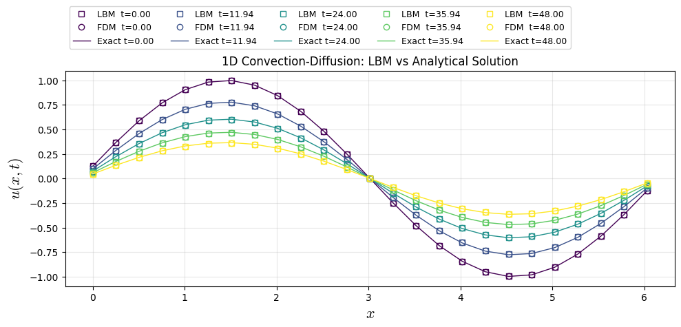
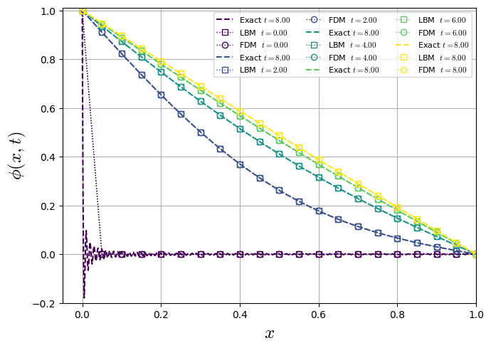
2nd Benchmark: Temperature ramp
Analyzing the accuracy of diffusive equation solver, we apply it to a one-dimensional analytical case. The geometry is described by a domain of length \(L\) initialized with a constant temperatura \(T(x,t=0)=0\). The boundary conditions are given \(T(x=0,t)=1\) and \(T(x=L,t)=0\).
Steady-State Analytical Solution
The analytical solution of this problem is given by:
Transient Analytical Solution
For the 1D heat equation \(\partial_t T=\nu\,\partial_{xx}T\) on \(0<x<L\) with
the steady state is \(T_{\text{ss}}(x)=1-\tfrac{x}{L}\). With \(u=T-T_{\text{ss}}\) (so \(u(0,t)=u(L,t)=0\)), the solution is
Special case \(T_0(x)=0\): \(B_n=-\dfrac{2}{n\pi}\), so
Here’s a ready-to-run Python snippet (with a single plot of \(T(x,t)\) vs \(x\) for multiple times):
LBM D1Q3 Code - FDM Code
Show code cell source
import warnings
warnings.filterwarnings("ignore")
import numpy as np
import matplotlib.pyplot as plt
import matplotlib
matplotlib.rcParams['mathtext.fontset'] = 'cm'
#--------------------------------------- Parameters (physical units) ------------------------------------------
L = 1.0             # Length of the domain
nu = 0.1/2.0        # Diffusion coefficient
t_end = 8.0             # Total simulation time
#--------------------------------------- Lattice-Properties-D1Q3 ----------------------------------------------
cs=1.0/np.sqrt(3.0);
w = np.array([4.0/6.0, 1.0/6.0, 1.0/6.0],dtype="float64")
cx = np.array([0, 1, -1],dtype="int8")
#------------------------------------- Parameters (numerical units) -------------------------------------------
Nx=21               # Domain Length
dx = L / (Nx-1)     # Spatial step size
c=1.0*2**(2)        # c=dx/dt
dt=dx/c             # Time step value
nt = int(t_end / dt)    # Time step number
nue=nu/(c*dx)       # Diffusion coefficient
tau=nue/cs**2+0.5   # Relaxation Time
omg=1.0/tau
print(f"dx={dx:.4e}\t dt={dt:.4e}\t nt={nt:d}") # Print values for check
print(f"nue={nue:.4f}\t tau={tau:.4f}\t omega={omg:.4f}")
#--------------------------------- Initialization - LBM - Numerical Arrays -----------------------------------------
T = np.zeros((Nx),dtype="float64")
T[0]=1.0 # Initital Temperature Field
f = np.zeros((3,Nx),dtype="float64")
fp = np.zeros((3,Nx),dtype="float64")
for k in range(0,3):
    f[k,:]=w[k]*T[:]
    fp[k,:]=w[k]*T[:]
#--------------------------------- Initialization - FDM - Numerical Arrays -----------------------------------------
Tfm2 = np.zeros((Nx),dtype="float64")    # Temperature field at the step t-2
Tfm = np.zeros((Nx),dtype="float64")    # Temperature field at the step t-1
Tf = np.zeros((Nx),dtype="float64")     # Temperature field at the step t
Tfp = np.zeros((Nx),dtype="float64")    # Temperature field at the step t+1
Tfm2[0]=1.0                              # Initital Temperature Field
Tfm[0]=1.0                              # Initital Temperature Field
Tf[0]=1.0                               # Initital Temperature Field
Tfp[0]=1.0                              # Initital Temperature Field
#--------------------------------- Initialization - Save Data Arrays -----------------------------------------
snaps=5 # number of states saved over time including 0 and t_end
T_snaps = np.empty(snaps, dtype=object) # array field used to same data over time
Tf_snaps = np.empty(snaps, dtype=object) # array field used to same data over time
snaps_id = np.linspace(0, nt, snaps, dtype="int16") # timesteps to take the field
snap_index = {sid: i for i, sid in enumerate(snaps_id)}
for i in range(snaps):
    T_snaps[i] = np.zeros((Nx), dtype="float64")
    Tf_snaps[i] = np.zeros((Nx), dtype="float64")
T_snaps[0][:]=T[:]
Tf_snaps[0][:]=Tf[:]
#----------------------------------------- Maind Loop --------------------------------------------------------
for t in range(nt):
    #========================================= LBM - Solution =============================================
    #--------------------Collision----------------
    for k in range(0,3):
        fp[k,:]=f[k,:] - (f[k,:] - w[k]*T[:])/tau
    #-----------------streaming-------------------
    for k in range(0,3):
        f[k,:]=np.roll(fp[k,:], cx[k], axis=0)
    #-----------------Boundaries-----------------------
    f[1,0]= 1.0 - f[0,0]-f[2,0]
    f[2,Nx-1]= 0.0 - f[0,Nx-1]-f[1,Nx-1]
    #----------------------Macro------------------
    T[:]=f[0,:]+f[1,:]+f[2,:]
    #---------------------save-snaps--------------
    if t+1 in snaps_id:
        i = snap_index[t+1]
        T_snaps[i][:]=T[:]
    #========================================= FDM - Solution =============================================
    if (t<2) :
        Tfm2[:]=Tfm[:]     # Swap for update t-1 to t-2
        Tfm[:]=Tf[:]     # Swap for update t to t-1
        Tf[:]=T[:]     # Swap for update t to t-1
    else :
        Tfp[:]=( ( (1-omg+omg*w[1])*np.roll(Tf[:],1,axis=0) + (1-omg+omg*w[0])*Tf[:] + (1-omg+omg*w[2])*np.roll(Tf[:],-1,axis=0) )
                 - (1-omg)**(2)*( np.roll(Tfm[:], 1, axis=0) + Tfm[:] + np.roll(Tfm[:], -1, axis=0) )
                 - (1-omg)*omg*( (w[0]+w[1])*np.roll(Tfm[:], 1, axis=0) + (w[2]+w[1])*Tfm[:] + (w[2]+w[0])*np.roll(Tfm[:], -1, axis=0) )
                 + (1.0-omg)**(2)*Tfm2[:]  )
        Tfp[0]=1.0
        Tfp[Nx-1]=0.0
        Tfm2[:]=Tfm[:]     # Swap for update t-1 to t-2
        Tfm[:]=Tf[:]     # Swap for update t to t-1
        Tf[:]=Tfp[:]     # Swap for update t+1 to t
    #---------------------save-snaps------------
    if t+1 in snaps_id:
        i = snap_index[t+1]
        Tf_snaps[i][:]=Tfp[:]
Show code cell output
dx=5.0000e-02	 dt=1.2500e-02	 nt=640
nue=0.2500	 tau=1.2500	 omega=0.8000
Show code cell source
import numpy as np
import matplotlib.pyplot as plt

# ---- Modes and series -------------------------------------------------------
def modes_dirichlet_dirichlet(L, N):
    n = np.arange(1, N+1)        # n = 1,2,...,N
    k = n * np.pi / L            # eigenvalues mu_n
    return n, k

def project_coeffs_dirichlet(T0_func, L, N, grid_pts=4000):
    """
    B_n = (2/L) ∫( T0(x) - T_ss(x) ) sin(nπx/L) dx, with T_ss = 1 - x/L.
    """
    x = np.linspace(0.0, L, grid_pts, endpoint=True)
    Tss = 1.0 - x / L
    u0 = T0_func(x) - Tss
    n, k = modes_dirichlet_dirichlet(L, N)          # (N,), (N,)
    S = np.sin(k[:, None] * x[None, :])             # (N, M)
    B = (2.0 / L) * np.trapz(u0[None, :] * S, x, axis=1)
    return B, n, k

def T_series_dirichlet(x, t, L, nu, B, k):
    """
    T(x,t) = T_ss(x) + sum_n B_n e^{-nu k_n^2 t} sin(k_n x), T_ss = 1 - x/L.
    """
    x = np.asarray(x)
    Tss = 1.0 - x / L
    coeff = B * np.exp(-nu * (k**2) * t)            # (N,)
    add = np.sum(coeff[:, None] * np.sin(k[:, None] * x[None, :]), axis=0)
    return Tss + add

# ---- Parameters -------------------------------------------------------------
L   = 1.0
nu  = 0.1/2.0
N   = 200
x   = np.linspace(0, L, 600)

# ---- Case A: initially cold rod T0(x)=0 (closed-form coefficients) ----------
n, k = modes_dirichlet_dirichlet(L, N)
B_cold = -2.0 / (n * np.pi)   # exact coefficients for T0 ≡ 0

times = [0.0, 2.0, 4.0, 6.0, 8.0]

#--------------------------------------- Plot Results -------------------------------------------------------
xl = np.linspace(0, L, Nx)
times = np.linspace(0, t_end, snaps, dtype="float64") # timesteps to take the field
plt.figure(figsize=(7, 5))
colors = plt.cm.viridis(np.linspace(0, 1, snaps))
for i in range(snaps):
    T_xt = T_series_dirichlet(x, times[i], L, nu, B_cold, k)
    plt.plot(x, T_xt, "--", color=colors[i], label=f"Exact $t = {t:.2f}$")
    plt.plot(xl, T_snaps[i], "s:", color=colors[i], lw=1, label=f"LBM  $t={(snaps_id[i]/nt)*t_end :.2f}$",fillstyle='none')
    plt.plot(xl, Tf_snaps[i], "o:", color=colors[i], lw=1, label=f"FDM  $t={(snaps_id[i]/nt)*t_end :.2f}$",fillstyle='none')
plt.xlabel(r"$x$",fontsize=18)
plt.ylabel(r"$\phi(x,t)$",fontsize=18)
plt.legend(ncol=3,fontsize=8)
plt.xlim(-0.05,1)
plt.ylim(-0.2,1.01)
plt.grid(True)
plt.tight_layout()
plt.show()
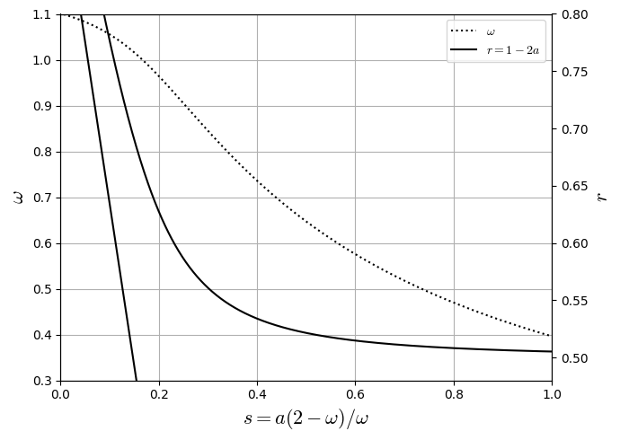
Fourth-order Diffusive Equation
Expanding the sums:
Considering $\( \alpha_{1}=\Omega + a\omega, \quad \alpha_{2}=\Omega + (1-2a)\omega, \quad \beta_{1}=-\Omega(\Omega + (1-a)\omega), \quad \textrm{and} \quad \beta_{2}=-\Omega(\Omega + 2a\omega), \)$
where \(\Omega=(1-\omega)\) and \(a=w_{1}=w_{2}\). Replacing in the Eq. (60):
To recover the partial differetial equation described by the above equation, we expand each \(\phi\) term in Taylor series:
Replacing the expanded terms and simplifying the term (this link provide a sympy code that reach the above equation Sympy code for FDM expansion of LBM diffusive equation), we have:
where \(\nu=\frac{a \left(2 - \omega \right)}{\omega} \frac{\Delta_{x}^{2}}{\Delta_{t}}\) is the same term recovered in the Chapman-Enskog Analysis. To enforce fourth-order \(\Delta_{x}\) convergence rate, employ the relations
Show code cell source
import warnings
warnings.filterwarnings("ignore")

import numpy as np
import matplotlib.pyplot as plt
import matplotlib
matplotlib.rcParams['mathtext.fontset'] = 'cm'

# ---- data ----
om = np.linspace(0.2, 1.5, 1000)
a  = (om**2 - 12*om + 12) / (6*(om**2 - 8*om + 8))
r  = 1.0 - 2.0*a
s  = a * (2.0 - om) / om

# ---- figure and axes ----
fig, ax1 = plt.subplots(figsize=(7, 5))

# Left y-axis: omega
ax1.plot(s, om, 'k:', label=r'$\omega$')
ax1.set_xlabel(r'$s = a(2-\omega)/\omega$',fontsize=16)
ax1.set_ylabel(r'$\omega$',fontsize=16)
ax1.set_ylim(0.3, 1.1)
ax1.set_xlim(0.0, 1.0)
ax1.grid(True)

# Right y-axis: r
ax2 = ax1.twinx()
ax2.plot(s, r, 'k-', label=r'$r = 1 - 2a$')
ax2.set_ylabel(r'$r$',fontsize=16)
ax2.set_ylim(0.48, 0.8)
ax2.set_xlim(0.0, 1.0)

# ---- combined legend ----
lines1, labels1 = ax1.get_legend_handles_labels()
lines2, labels2 = ax2.get_legend_handles_labels()
ax1.legend(lines1 + lines2, labels1 + labels2, loc='best')

plt.tight_layout()
plt.show()
Show code cell source
import warnings
warnings.filterwarnings("ignore")
import numpy as np
import matplotlib.pyplot as plt
import matplotlib
matplotlib.rcParams['mathtext.fontset'] = 'cm'
matplotlib.rcParams['mathtext.fontset'] = 'cm'
#--------------------------------------- Parameters (physical units) ------------------------------------------
A   = 1.0                         # Amplitude
phi = 0.0                         # Wave initial shift
k_w   = 1.0                       # Wave number
c   = 0.0                         # wave speed
nu  = 0.066666666666666666*np.pi # Diffusive coefficient
m_waves = 1                       # Wave Period
L = m_waves * (2.0*np.pi / k_w)   # Domain Lentgh
t_end = 12.0                       # Final time
#--------------------------------------- Lattice-Properties-D1Q3 ----------------------------------------------
w = np.array([4.0/6.0, 1.0/6.0, 1.0/6.0],dtype="float64")
cx = np.array([0, 1, -1],dtype="int16")
cs=1.0/np.sqrt(3.0);
#--------------------------------- Initialization - Save Data Arrays -----------------------------------------------
cases=4
Nx0 = np.array([10, 20, 40, 80],dtype="int64")
r0 = 2**(0)*np.array([2.0**(1), 2.0**(2), 2.0**(3), 2.0**(4)],dtype="float64")
u_cases = np.empty(cases, dtype=object) # array field used to same data over time
for i in range(cases):
    u_cases[i] = np.zeros((Nx0[i]), dtype="float64")
for case in range(0,cases):
    #------------------------------------- Parameters (numerical units) -------------------------------------------
    Nx=Nx0[case]  # Numerical Length
    x  = np.linspace(0.0, L, Nx, endpoint=False,dtype="float64") # Numerical Domain
    dx = L / Nx # Grid size
    r = 1*r0[case] # dx/dt relation
    dt = dx/r
    ce = c/r
    nue = nu * dt / (dx*dx)
    tau = 0.5 + nue / cs**2
    omg=1.0/tau
    nt = int(np.ceil(t_end / dt))
    print(f"dx={dx:.4e}\t dt={dt:.4e}\t nt={nt:d}\t tn={nt*dt:.2f}") # Print values for check
    print(f"c_lbm={ce:.3f}, tau={tau:.4f}\t omega={omg:.2f}")
    print(f"nt={nt:.3f}, nue={nue:.4f}")
    #--------------------------------- Initialization - LBM - Numerical Arrays -----------------------------------------
    u=np.zeros((Nx),dtype="float64")
    u = A * np.sin(k_w*(x+dx/2) + phi)
    f=np.zeros((3,Nx),dtype="float64")
    fp=np.zeros((3,Nx),dtype="float64")
    for k in range(0,3):
        f[k,:]=w[k]*(u[:]+cx[k]*ce*u[:]/cs**2)
        fp[k,:]=w[k]*(u[:]+cx[k]*ce*u[:]/cs**2)
    #----------------------------------------- Maind Loop --------------------------------------------------------
    for t in range(nt):
        #========================================= LBM - Solution =============================================
        #--------------------Collision----------------
        for k in range(0,3):
            fp[k,:]= f[k,:] - (f[k,:] - w[k]*(u[:]+cx[k]*(ce*u[:])/cs**2))/tau
        #-----------------streaming-------------------
        for k in range(0,3):
            f[k,:]=np.roll(fp[k,:], cx[k], axis=0)
        #----------------------Macro------------------
        u[:]=f[0,:]+f[1,:]+f[2,:]
    #---------------------save-field-cases--------------
    u_cases[case][:]=u[:]
Show code cell output
dx=6.2832e-01	 dt=3.1416e-01	 nt=39	 tn=12.25
c_lbm=0.000, tau=1.0000	 omega=1.00
nt=39.000, nue=0.1667
dx=3.1416e-01	 dt=7.8540e-02	 nt=153	 tn=12.02
c_lbm=0.000, tau=1.0000	 omega=1.00
nt=153.000, nue=0.1667
dx=1.5708e-01	 dt=1.9635e-02	 nt=612	 tn=12.02
c_lbm=0.000, tau=1.0000	 omega=1.00
nt=612.000, nue=0.1667
dx=7.8540e-02	 dt=4.9087e-03	 nt=2445	 tn=12.00
c_lbm=0.000, tau=1.0000	 omega=1.00
nt=2445.000, nue=0.1667
Show code cell source
#****************************************Data-Analysis*********************************************
# ---------------- exact solution ----------------
def u_exact(x, t, A, k_w, phi, c, nu):
return A * np.exp(-nu * k_w**2 * t) * np.sin(k_w * ((x+dx/2) - c*t) + phi)
u_ana = np.empty(cases, dtype=object) # array field used to same data over time
xl = np.empty(cases, dtype=object) # array field used to same data over time
for i in range(cases):
Nx=Nx0[i] # Numerical Length
x = np.linspace(0.0, L, Nx, endpoint=False,dtype="float64") # Numerical Domain
dx = L / Nx # Grid size
r = r0[i] # dx/dt relation
dt = dx/r
nt = int(np.ceil(t_end / dt))
xl[i] = np.linspace(0.0, L, Nx0[i], endpoint=False,dtype="float64")
u_ana[i] = np.zeros((Nx0[i]), dtype="float64")
u_ana[i] = u_exact(xl[i], nt*dt , A, k_w, phi, c, nu)
# -----------------Plot Results --------------------
plt.figure(figsize=(10,5))
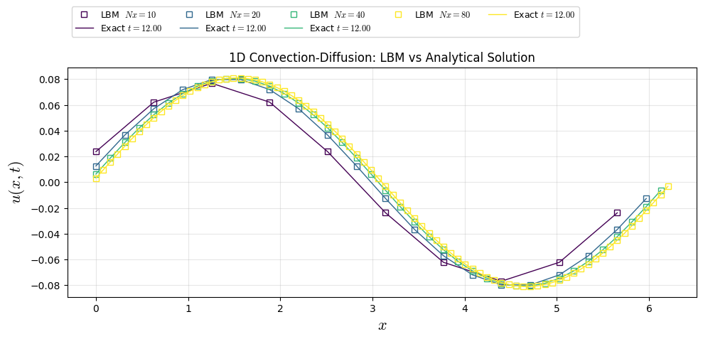
colors = plt.cm.viridis(np.linspace(0, 1, cases))
for i in range(cases):
plt.plot(xl[i], u_cases[i], "s", color=colors[i], lw=1, label=f"LBM $Nx={Nx0[i]:.0f}$",fillstyle='none')
plt.plot(xl[i], u_ana[i], color=colors[i], lw=1, label=f"Exact $t={t_end:.2f}$")
plt.xlabel("$x$",fontsize=16)
plt.ylabel("$u(x,t)$",fontsize=16)
plt.title("1D Convection-Diffusion: LBM vs Analytical Solution")
plt.grid(True, alpha=0.3)
plt.legend(ncol=5,fontsize=9,loc="center left",bbox_to_anchor=(0.0, 1.2))
plt.tight_layout()
plt.show()
Show code cell source
Erro= np.zeros((cases), dtype="float64")
for i in range(cases):
    Erro[i]=np.sqrt(np.sum((u_cases[i]-u_ana[i])**2))/np.sqrt(np.sum((u_ana[i])**2))
    print(f'Erro{i}=',Erro[i])
TEp=np.polyfit(np.log(Nx0), np.log(Erro), 1)
print(TEp)
print(f'ltests[i] = np.array([{1/tau:.2f},{cs**2:.2f},{-TEp[0]:.2f},{Erro[0]},{Erro[1]},{Erro[2]},{Erro[3]}],dtype="float64")')
Show code cell output
Erro0= 0.0007675056151646606
Erro1= 4.5801886601000255e-05
Erro2= 2.843695561303167e-06
Erro3= 1.772197264107726e-07
[-4.02508353  2.08310237]
ltests[i] = np.array([1.00,0.33,4.03,0.0007675056151646606,4.5801886601000255e-05,2.843695561303167e-06,1.772197264107726e-07],dtype="float64")
Show code cell source
#------------------ List of teste cases ---------------------------
ntests=7
ltests = np.empty(ntests, dtype=object) # list [omega, cs**2, a, erro1, erro2, erro3]
ltests[0] = np.array([1.00,0.33,4.03,0.0007675056151646606,4.5801886601000255e-05,2.843695561303167e-06,1.772197264107726e-07],dtype="float64")
ltests[1] = np.array([1.33,0.33,1.98,0.14172076082874474,0.03676563394470728,0.00926664086838909,0.0023217597555758216],dtype="float64")
ltests[2] = np.array([1.60,0.33,1.97,0.173048134806591,0.045658664282350235,0.011566406970317222,0.002901017675903232],dtype="float64")
ltests[3] = np.array([1.78,0.33,1.96,0.1806210735638166,0.04785433656697225,0.012139180249442527,0.003045785275804],dtype="float64")
ltests[4] = np.array([0.67,0.33,2.12,0.4515322151274699,0.09291589762687379,0.022049149483031594,0.005442330222168221],dtype="float64")
ltests[5] = np.array([0.40,0.33,2.19,2.5815332944176905,0.5537880973820454,0.11602188228229841,0.02759320543861061],dtype="float64")
ltests[6] = np.array([0.22,0.33,1.80,4.667938739917,2.687002267460583,0.5746533215752334,0.1219574567471747],dtype="float64")
Show code cell source
matplotlib.rcParams['mathtext.fontset'] = 'cm'
plt.figure(figsize=(7,4))
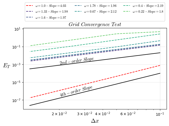
plt.title("$Grid$ $Convergence$ $Test$",fontsize=14)
colors = plt.cm.viridis(np.linspace(0, 1, ntests-1))
plt.loglog(1/Nx0,ltests[0][3:],'r--',fillstyle='none', label=f'$\\omega={ltests[0][0]}$ - $Slope={ltests[0][2]}$')
for i in range(7)[1:]:
plt.loglog(1/Nx0,ltests[i][3:],'--',color=colors[i],fillstyle='none', label=f'$\\omega={ltests[i][0]}$ - $Slope={ltests[i][2]}$')
plt.loglog(1/Nx0,2.*1.0/(Nx0**2),'k-',fillstyle='none')
plt.text(0.02, 0.001, "$2nd-order$ $Slope$", rotation=8,fontsize=12)
plt.loglog(1/Nx0,1.*1.0/(Nx0**4),'k-',fillstyle='none')
plt.text(0.02, 0.00000025, "$4th-order$ $Slope$", rotation=15,fontsize=12)
# plt.ylim(0,0.01)
plt.grid(True, alpha=0.3)
# plt.legend(loc=2,ncol=3,fontsize=8.5)
plt.legend(ncol=3,fontsize=9,loc="center left",bbox_to_anchor=(0.0, 1.2))
plt.ylabel('$E_{T}$',fontsize=16,rotation=0,horizontalalignment='right')
plt.xlabel('$\Delta x$',fontsize=16)
plt.show()
Extension for Higher-Dimensions and Anisotropy
Suga [9] also extend the approach for 2 and 3D cases considering anisotropic scenarios. Notice that different second order errors will appear with other dimensions:
Interpretation for Diffusive Equation in a MRT-Framework
Extending the approach Developed above for now considering a sistems of multiple relaxatio time. The present development follow sequence presente in Lin et al. [10].
Show code cell source
import warnings
warnings.filterwarnings("ignore")
from pylab import *
from sympy import *
import numpy as np

fic, f0c, f1c, f2c = symbols(['f_{i\,x+c_{i}}^t','f_{0\,x+c_{i}}^t','f_{1\,x+c_{i}}^t','f_{2\,x+c_{i}}^t'])
f0tp1, f1tp1, f2tp1 = symbols(['f_{0\,x}^{t+1}','f_{1\,x}^{t+1}','f_{2\,x}^{t+1}'])
f0, f1, f2 = symbols(['f_{0\,x}^t','f_{1\,x}^t','f_{2\,x}^t'])
f0m1, f1m1, f2m1, f0p1, f1p1, f2p1 = symbols(['f_{0\,x-1}^t','f_{1\,x-1}^t','f_{2\,x-1}^t','f_{0\,x+1}^t','f_{1\,x+1}^t','f_{2\,x+1}^t'])
f0m1t1, f1m1t1, f2m1t1, f0p1t1, f1p1t1, f2p1t1 = symbols(['f_{0\,x-1}^{t-1}','f_{1\,x-1}^{t-1}','f_{2\,x-1}^{t-1}','f_{0\,x+1}^{t-1}','f_{1\,x+1}^{t-1}','f_{2\,x+1}^{t-1}'])
f0t1 = symbols('f_{0\,x}^{t-1}')
w0, w1, w2 = symbols(['w_0','w_1','w_2'])
s0, s1, s2 = symbols(['s_0','s_1','s_2'])
phi, phic, phim1, phip1 = symbols(['\\phi_{x}^{t}','\\phi_{x-c_{i}}^{t}','\\phi_{x-1}^{t}','\\phi_{x+1}^{t}'])
phitp1, phit1, phit2= symbols(['\\phi_{x}^{t+1}','\\phi_{x}^{t-1}','\\phi_{x}^{t-2}'])
phim1t1,phip1t1= symbols(['\\phi_{x-1}^{t-1}','\\phi_{x+1}^{t-1}'])
cx=np.array([0,1,-1])
wi=np.array([w0,w1,w2])
wiM=Matrix([w0,w1,w2])
fi=np.array([f0,f1,f2])
fM = Matrix([f0,f1,f2])
ficM = Matrix([f0c,f1c,f2c])
feq=phi*wi
feqM=Matrix([feq[0],feq[1],feq[2]])
feqc=wiM*phic
Show code cell source
m0=np.array([1,1,1])
m1=cx
m2=3*cx*cx - 2
M=np.array([m0,m1,m2])
MM=Matrix([m0,m1,m2])
MM
Show code cell source
Meq=np.array([simplify(sum(feq*M[0])), simplify(sum(feq*M[1])), simplify(sum(feq*M[2]))])
MeqM=Matrix([simplify(sum(feq*M[0])), simplify(sum(feq*M[1])), simplify(sum(feq*M[2]))])
MeqM
Show code cell source
I=eye(3)
S=np.array([I[0,:]*s0,I[1,:]*s1,I[2,:]*s2])
SM=Matrix([I[0,:]*s0,I[1,:]*s1,I[2,:]*s2])
SM
Show code cell source
MMinv=MM.inv()
MMinv
Show code cell source
display(MMinv*(SM*(MM*(ficM))))
Show code cell source
PM=ficM-MMinv*(SM*(MM*(ficM-feqc)))
display(Eq(ficM,PM))
Show code cell source
fp0=simplify(collect(PM[0].subs(phic,phi),phi).subs({f0c:f0,f1c:f1,f2c:f2}).subs({-w0-w1-w2:-1,f0+f1+f2:phi,f1+f2:-f0+phi,-w1-w2:-1+w0}))
Eq(f0tp1,fp0)
Show code cell source
fp1=simplify(collect(PM[1].subs(phic,phim1),phim1).subs({f0c:f0m1,f1c:f1m1,f2c:f2m1}).subs({-w0-w1-w2:-1,f0m1+f1m1+f2m1:phim1,-w1-w2:-1+w0})
                    .subs({f1m1+f2m1:phim1-f0m1,w1-w2:0}) )
Eq(f1tp1,fp1)
Show code cell source
fp2=simplify(collect(PM[2].subs(phic,phip1),phip1).subs({f0c:f0p1,f1c:f1p1,f2c:f2p1}).subs({-w0-w1-w2:-1,f0p1+f1p1+f2p1:phip1,-w1-w2:-1+w0})
                    .subs({f1p1+f2p1:phip1-f0p1,w1-w2:0}) )
Eq(f2tp1,fp2)
Show code cell source
term1=collect(fp0+fp1+fp2,[w0*s2,s2,s1/2])
Eq(phitp1,term1)
Reinterpreting the above equation, we can derive
Show code cell source
term2=collect(fp0+fp1+fp2,[w0*s2,s2,s1/2]).subs(f1p1,phit1-f0-f2m1).subs(f1p1,phit1-f0-f2m1)
Eq(phitp1,term2)
To repalce the term \(f_{0,x}^{t}+f_{1,x-1}^{t}+f_{2,x+1}^{t}\), in the above equation we use the \(\sum_{i}f_{i,x}^{t}=\phi_{x}^{t}\):
Show code cell source
rel2=(f0+f1m1+f2p1).subs(f1m1,phim1-f0m1-f2m1).subs(f2p1,phip1-f0p1-f1p1).subs(-f1p1-f2m1,f0-phit1)
Eq(f0+f1m1+f2p1,rel2)
Show code cell source
term3=collect(fp0+fp1+fp2,[w0*s2,s2,s1/2]).subs(f1p1,phit1-f0-f2m1).subs(f1p1,phit1-f0-f2m1).subs(-f0-f1m1-f2p1,-rel2)
term4=collect(collect(expand(term3),[f0m1,f0,f0p1,phip1,phim1,phit1]).subs(f0*(-s1-s2+2),-2*f0*(s1/2+s2/2-1)),(s1/2+s2/2-1))
Eq(phitp1,term4)
Show code cell source
rel3=(-2*f0+f0m1+f0p1).subs(-2*f0,-2*phi + 2*f1+ 2*f2)
Eq(-2*f0+f0m1+f0p1,rel3)
Replace the distribution functions in above relation by your collisional form
Show code cell source
rel3s1=collect(rel3.subs(f0p1,phip1t1*s2*w0-f0p1t1*s2+f0p1t1).subs(f0m1,phim1t1*s2*w0-f0m1t1*s2+f0m1t1).subs(f1,-phim1t1*s2*w0/2+f0m1t1*s2/2+f1m1t1+s1/2*(f2m1t1-f1m1t1))
       .subs(f2,-phip1t1*s2*w0/2+f0p1t1*s2/2+f2p1t1+s1/2*(f1p1t1-f2p1t1)),s1)
Eq(-2*f0+f0m1+f0p1,rel3s1)
Replacing in the above relation the terms \(f_{1,x-1}^{t-1}\) and \(f_{2,x+1}^{t-1}\) usgin Eq. (61):
Show code cell source
rel3s2=(rel3s1.subs(f1m1t1,phim1t1-f0m1t1-f2m1t1).subs(f2p1t1,phip1t1-f0p1t1-f1p1t1))
display(Eq(-2*f0+f0m1+f0p1,rel3s2))
Show code cell source
rel3s3=collect(simplify(collect(expand(rel3s2.subs(f2m1t1,phit2-f0t1-f1p1t1)),[f0p1t1,f0m1t1,2*f0t1,phim1t1,phip1t1,phit2])),[s1-1])
display(Eq(-2*f0+f0m1+f0p1,rel3s3))
Replacing the above relation in \(\phi_{x}^{t+1}\) term:
Show code cell source
term5=simplify(collect(expand(term4.subs(-2*f0+f0m1+f0p1,rel3s3)),[phim1,phip1,phim1t1,phip1t1,phit1,phit2,phi,f0p1t1,f0m1t1,f0t1]))
term5s1=collect(term5,[s1*s1+s1*s2-3*s1-s2+2,s1+w0*s2-2,s1*s1+s1*s2-4*s1-2*s2+4]).subs(s1*s1+s1*s2-3*s1-s2+2,(s1-1)*(s1+s2-2))
Eq(phitp1,term5s1)
Applying a shift in time for the Eq. XX.
Show code cell source
term6=simplify(expand(term5s1.subs( -f0t1+f0m1t1/2+f0p1t1/2, (phi-(phip1t1+phim1t1)*(1-s1/2-s2*w0/2) - phit2*(s1-1) - phit1*s2*w0)/(s1+s2-2) ) ))
Eq(phitp1,term6)
Show code cell source
collect(term6,[phim1,phip1,phi,phim1t1,phip1t1,phit1,phit2])
Fourth-order MRT Diffusive Equation
To recover the partial differetial equation with Fourth-order of convergence error, we expand each \(\phi\) term in Taylor series (this link provide a sympy code that reach the above equation Sympy code for FDM expansion of LBM diffusive equation up to Fourth-order):
Considering diffusive coeficient \(\nu=(1-w_{0})\left(\frac{1}{s_{1}} - \frac{1}{2}\right)\frac{\Delta_{x}^{2}}{\Delta_{t}}\), we can rewrite the equation
Using the relations:
we can reduce the equation in terms of \(\frac{\partial^{4}\phi}{\partial x^{4}}\):
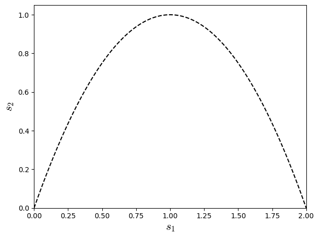
Making the term \(\left(3 s_{1}^{2} s_{2} w_{0} - 2 s_{1}^{2} s_{2} - 6 s_{1}^{2} w_{0} - 18 s_{1} s_{2} w_{0} + 12 s_{1} s_{2} + 12 s_{1} w_{0} + 12 s_{2} w_{0} - 12 s_{2}\right)\) equal to zero e can reach fourth order approximation. For \(w_{0}=2/3\) (weight specific from the lattice D1Q3) the relation reduce to \(4s_{1}^{2} -8s_{1}+4s_{2}\):
Show code cell source
import warnings
warnings.filterwarnings("ignore")

import numpy as np
import matplotlib.pyplot as plt
import matplotlib
matplotlib.rcParams['mathtext.fontset'] = 'cm'

# ---- data ----
s1r = np.linspace(0, 2.0, 1000)
s2r  = s1r*(2-s1r)

plt.plot(s1r,s2r,'k--')
plt.xlabel(r'$s_{1}$',fontsize=16)
plt.ylabel(r'$s_{2}$',fontsize=16)
plt.xlim(0,2)
plt.ylim(0,1.05)

plt.tight_layout()
plt.show()
Show code cell source
import warnings
warnings.filterwarnings("ignore")
import numpy as np
import matplotlib.pyplot as plt
import matplotlib
matplotlib.rcParams['mathtext.fontset'] = 'cm'
matplotlib.rcParams['mathtext.fontset'] = 'cm'
#--------------------------------------- Parameters (physical units) ------------------------------------------
A   = 1.0                         # Amplitude
phi = 0.0                         # Wave initial shift
k_w   = 1.0                       # Wave number
c   = 0.0                         # wave speed
nu  = 0.066666666666666666*np.pi # Diffusive coefficient
m_waves = 1                       # Wave Period
L = m_waves * (2.0*np.pi / k_w)   # Domain Lentgh
t_end = 12.0                       # Final time
#--------------------------------------- Lattice-Properties-D1Q3 ----------------------------------------------
w = np.array([4.0/6.0, 1.0/6.0, 1.0/6.0],dtype="float64")
cx = np.array([0, 1, -1],dtype="int16")
cs=1.0/np.sqrt(3.0);
#--------------------------------- Initialization - Save Data Arrays -----------------------------------------------
cases=4
Nx0 = np.array([10, 20, 40, 80],dtype="int64")
r0 = 2**(0)*np.array([2.0**(1), 2.0**(2), 2.0**(3), 2.0**(4)],dtype="float64")
u_cases = np.empty(cases, dtype=object) # array field used to same data over time
for i in range(cases):
    u_cases[i] = np.zeros((Nx0[i]), dtype="float64")
for case in range(0,cases):
    #------------------------------------- Parameters (numerical units) -------------------------------------------
    Nx=Nx0[case]  # Numerical Length
    x  = np.linspace(0.0, L, Nx, endpoint=False,dtype="float64") # Numerical Domain
    dx = L / Nx # Grid size
    r = 1*r0[case] # dx/dt relation
    dt = dx/r
    ce = c/r
    nue = nu * dt / (dx*dx)
    tau1 = 0.5 + nue / cs**2
    tau2=1.0/((1.0/tau1)*(2.0-(1.0/tau1)))
    nt = int(np.ceil(t_end / dt))
    print(f"dx={dx:.4e},\t dt={dt:.4e}\t nt={nt:d},\t tn={nt*dt:.2f}") # Print values for check
    print(f"c_lbm={ce:.3f},\t tau1={tau1:.4f},\t tau2={tau2:.4f}")
    print(f"s1={1.0/tau1:.4f},\t s2={1.0/tau2:.4f}")
    print(f"nt={nt:.3f}\t, nue={nue:.4f}")
    #--------------------------------- Initialization - LBM - Numerical Arrays -----------------------------------------
    u=np.zeros((Nx),dtype="float64")
    u = A * np.sin(k_w*(x+dx/2) + phi)
    mx=np.zeros((Nx),dtype="float64")
    mxx=np.zeros((Nx),dtype="float64")
    f=np.zeros((3,Nx),dtype="float64")
    feq=np.zeros((3,Nx),dtype="float64")
    fp=np.zeros((3,Nx),dtype="float64")
    for k in range(0,3):
        f[k,:]=w[k]*(u[:]+cx[k]*ce*u[:]/cs**2)
        fp[k,:]=w[k]*(u[:]+cx[k]*ce*u[:]/cs**2)
    #----------------------------------------- Init Loop --------------------------------------------------------
    for t in range(nt*10):
        #========================================= LBM - Solution =============================================
        #--------------------Collision----------------
        for k in range(0,3):
            feq[k,:]= w[k]*(u[:]+cx[k]*(ce*u[:])/cs**2)
        mx = np.einsum('i,ix->x', cx, f-feq)
        mxx = np.einsum('i,ix->x', 3.0*cx*cx-2.0, f-feq)
        for k in range(0,3):
            # fp[k,:]= f[k,:] - w[k]*( cx[k]*mx[:]/(tau1*cs**2) + (cx[k]**2-cs**2)*mxx[:]/(2.0*cs**2*tau2) )
            fp[k,:]= feq[k,:] + w[k]*( (1.0-1.0/tau1)*cx[k]*mx[:]/cs**2 + (1.0-1.0/tau2)*(cx[k]**2-cs**2)*mxx[:]/(2.0*cs**2) )
        #-----------------streaming-------------------
        for k in range(0,3):
            f[k,:]=np.roll(fp[k,:], cx[k], axis=0)
    #----------------------------------------- Maind Loop --------------------------------------------------------
    for t in range(nt):
        #========================================= LBM - Solution =============================================
        #--------------------Collision----------------
        for k in range(0,3):
            feq[k,:]= w[k]*(u[:]+cx[k]*(ce*u[:])/cs**2)
        mx = np.einsum('i,ix->x', cx, f-feq)
        mxx = np.einsum('i,ix->x', 3.0*cx*cx-2.0, f-feq)
        for k in range(0,3):
            # fp[k,:]= f[k,:] - w[k]*( cx[k]*mx[:]/(tau1*cs**2) + (cx[k]**2-cs**2)*mxx[:]/(2.0*cs**2*tau2) )
            fp[k,:]= feq[k,:] + w[k]*( (1.0-1.0/tau1)*cx[k]*mx[:]/cs**2 + (1.0-1.0/tau2)*(cx[k]**2-cs**2)*mxx[:]/(2.0*cs**2) )
        #-----------------streaming-------------------
        for k in range(0,3):
            f[k,:]=np.roll(fp[k,:], cx[k], axis=0)
        #----------------------Macro------------------
        # u[:]=f[0,:]+f[1,:]+f[2,:]
        u=np.einsum('ix->x', f)
    #---------------------save-field-cases--------------
    u_cases[case][:]=u[:]
Show code cell output
dx=6.2832e-01,	 dt=3.1416e-01	 nt=39,	 tn=12.25
c_lbm=0.000,	 tau1=1.0000,	 tau2=1.0000
s1=1.0000,	 s2=1.0000
nt=39.000	, nue=0.1667
dx=3.1416e-01,	 dt=7.8540e-02	 nt=153,	 tn=12.02
c_lbm=0.000,	 tau1=1.0000,	 tau2=1.0000
s1=1.0000,	 s2=1.0000
nt=153.000	, nue=0.1667
dx=1.5708e-01,	 dt=1.9635e-02	 nt=612,	 tn=12.02
c_lbm=0.000,	 tau1=1.0000,	 tau2=1.0000
s1=1.0000,	 s2=1.0000
nt=612.000	, nue=0.1667
dx=7.8540e-02,	 dt=4.9087e-03	 nt=2445,	 tn=12.00
c_lbm=0.000,	 tau1=1.0000,	 tau2=1.0000
s1=1.0000,	 s2=1.0000
nt=2445.000	, nue=0.1667
Show code cell source
#****************************************Data-Analysis*********************************************
# ---------------- exact solution ----------------
def u_exact(x, t, A, k_w, phi, c, nu):
    return A * np.exp(-nu * k_w**2 * t) * np.sin(k_w * ((x+dx/2) - c*t) + phi)
u_ana = np.empty(cases, dtype=object) # array field used to same data over time
xl = np.empty(cases, dtype=object) # array field used to same data over time
for i in range(cases):
    Nx=Nx0[i]  # Numerical Length
    x  = np.linspace(0.0, L, Nx, endpoint=False,dtype="float64") # Numerical Domain
    dx = L / Nx # Grid size
    r = r0[i] # dx/dt relation
    dt = dx/r
    nt = int(np.ceil(t_end / dt))
    xl[i] = np.linspace(0.0, L, Nx0[i], endpoint=False,dtype="float64")
    u_ana[i] = np.zeros((Nx0[i]), dtype="float64")
    u_ana[i] = u_exact(xl[i], nt*dt , A, k_w, phi, c, nu)
# -----------------Plot Results --------------------
plt.figure(figsize=(10,5))
colors = plt.cm.viridis(np.linspace(0, 1, cases))
for i in range(cases):
    plt.plot(xl[i], u_cases[i], "s", color=colors[i], lw=1, label=f"LBM  $Nx={Nx0[i]:.0f}$",fillstyle='none')
    plt.plot(xl[i], u_ana[i], color=colors[i], lw=1, label=f"Exact $t={t_end:.2f}$")

plt.xlabel("$x$",fontsize=16)
plt.ylabel("$u(x,t)$",fontsize=16)
plt.title("1D Convection-Diffusion: LBM vs Analytical Solution")
plt.grid(True, alpha=0.3)
plt.legend(ncol=5,fontsize=9,loc="center left",bbox_to_anchor=(0.0, 1.2))
plt.tight_layout()
plt.show()
Show code cell source
Erro= np.zeros((cases), dtype="float64")
for i in range(cases):
    Erro[i]=np.sqrt(np.sum((u_cases[i]-u_ana[i])**2))/np.sqrt(np.sum((u_ana[i])**2))
    print(f'Erro{i}=',Erro[i])
TEp=np.polyfit(np.log(Nx0), np.log(Erro), 1)
print(TEp)
print(f'ltests[i] = np.array([{1/tau1:.2f},{cs**2:.2f},{-TEp[0]:.2f},{Erro[0]},{Erro[1]},{Erro[2]},{Erro[3]}],dtype="float64")')
Show code cell output
Erro0= 0.0007675056151644276
Erro1= 4.580188660075553e-05
Erro2= 2.84369556091393e-06
Erro3= 1.7721972578567817e-07
[-4.02508353  2.08310237]
ltests[i] = np.array([1.00,0.33,4.03,0.0007675056151644276,4.580188660075553e-05,2.84369556091393e-06,1.7721972578567817e-07],dtype="float64")
Show code cell source
#------------------ List of teste cases ---------------------------
ntests=7
ltests = np.empty(ntests, dtype=object) # list [omega, cs**2, a, erro1, erro2, erro3]
ltests[0] = np.array([1.00,0.33,4.03,0.0007675056151646606,4.5801886601000255e-05,2.843695561303167e-06,1.772197264107726e-07],dtype="float64")
ltests[1] = np.array([1.33,0.33,4.00,0.0005319361354470807,3.3129765953764316e-05,2.0679546121974942e-06,1.2921092318928152e-07],dtype="float64")
ltests[2] = np.array([1.60,0.33,4.08,5.860129798788711e-05,3.189703761917948e-06,1.931515584995748e-07,1.196493783881998e-08],dtype="float64")
ltests[3] = np.array([1.78,0.33,3.99,0.0002483413735518823,1.579458417941352e-05,9.910176963429327e-07,6.199383613392777e-08],dtype="float64")
ltests[4] = np.array([0.67,0.33,4.02,0.03555687087757651,0.002131864590352776,0.00013235766481817078,8.263390671807474e-06],dtype="float64")
ltests[5] = np.array([0.40,0.33,4.05,0.5815809299211789,0.03474238662797822,0.0020727393050372516,0.00012853963043932504],dtype="float64")
ltests[6] = np.array([0.22,0.33,3.64,3.3399608313842446,0.5520470158617199,0.031960605145718385,0.0019041931043053725],dtype="float64")
Show code cell source
matplotlib.rcParams['mathtext.fontset'] = 'cm'
plt.figure(figsize=(7,4))
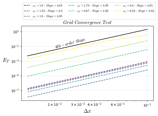
plt.title("$Grid$ $Convergence$ $Test$",fontsize=14)
colors = plt.cm.viridis(np.linspace(0, 1, ntests))
# plt.loglog(1/Nx0,ltests[0][3:],'r--',fillstyle='none', label=f'$\\omega={ltests[0][0]}$ - $Slope={ltests[0][2]}$')
for i in range(7):
plt.loglog(1/Nx0,ltests[i][3:],'--',color=colors[i],fillstyle='none', label=f'$\\omega_{1}={ltests[i][0]}$ - $Slope={ltests[i][2]}$')
plt.loglog(1/Nx0,1.*200000.0/(Nx0**4),'k-',fillstyle='none')
plt.text(0.02, 0.05, "$4th-order$ $Slope$", rotation=15,fontsize=12)
# plt.ylim(0,0.01)
plt.grid(True, alpha=0.3)
# plt.legend(loc=2,ncol=3,fontsize=8.5)
plt.legend(ncol=3,fontsize=9,loc="center left",bbox_to_anchor=(0.0, 1.2))
plt.ylabel('$E_{T}$',fontsize=16,rotation=0,horizontalalignment='right')
plt.xlabel('$\Delta x$',fontsize=16)
plt.show()
Sixth-order MRT Diffusive Equation
Extending up to Sixth-order of convergence error (this link provide a sympy code that reach the above equation Sympy code for FDM expansion of LBM diffusive equation up to Sixth-order):
where \(R^{4th}\) and \(R^{6th}\) are the terms in fouth and sixth-order error, respectively, given by:
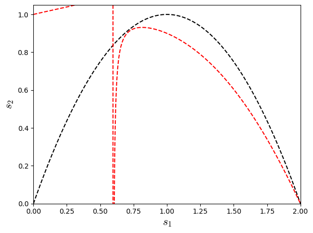
Making the term \(\left(3 s_{1}^{2} s_{2} w_{0} - 2 s_{1}^{2} s_{2} - 6 s_{1}^{2} w_{0} - 18 s_{1} s_{2} w_{0} + 12 s_{1} s_{2} + 12 s_{1} w_{0} + 12 s_{2} w_{0} - 12 s_{2}\right)\) equal to zero e can reach fourth order approximation. For \(w_{0}=2/3\) (weight specific from the lattice D1Q3) the relation reduce to \(4s_{1}^{2} -8s_{1}+4s_{2}\):
Trying to make both \(R^{4th}\) and \(R^{6th}\) null for lattice D1Q3 (\(w_{0}=2/3\)), we have the relation:
Show code cell source
import warnings
warnings.filterwarnings("ignore")

import numpy as np
import matplotlib.pyplot as plt
import matplotlib
matplotlib.rcParams['mathtext.fontset'] = 'cm'

# ---- data ----
s1r = np.linspace(0, 2.0, 1000)
s2r4  = s1r*(2.0-s1r)

s2r6  = (3.0*(2.0-s1r)*(s1r**2.0 + 6.0*s1r - 4.0))/(2.0*(2.0*s1r**3 - 11.0*s1r**2 + 26.0*s1r - 12.0))

plt.plot(s1r,s2r4,'k--')
plt.plot(s1r,s2r6,'r--')
plt.xlabel(r'$s_{1}$',fontsize=16)
plt.ylabel(r'$s_{2}$',fontsize=16)
plt.xlim(0,2)
plt.ylim(0,1.05)

plt.tight_layout()
plt.show()