Difference Finite Scheme derived from MRT Lattice Boltzmann for Convective-Diffusive Equation
Based on the works of Bellotti et al. [7] and Chen et al. [8], we will develop a difference finite description of lattice Boltzmann equation in the multi-relaxation-times (MRT) framework.
MRT Lattice Boltzmann equation for Convective-Diffusive Equation
To describe convective-diffusive problems, the MRT lattice Boltzmann formulation is described by:
where \(\textbf{M}\) is matrix of moments, \(\textbf{S}\) is the diagonal matrix of relaxation times, and \(\textbf{M}^{-1}\) is the inverse matrix of \(\textbf{M}\). Considering the problem description in a lattice D1Q3, we have:
The equilibrium distribution function is defined by
where \(\Lambda_{\alpha\beta}\) is a correction term defined by
Show code cell source
import warnings
warnings.filterwarnings("ignore")
from pylab import *
from __future__ import division
from sympy import *
import numpy as np
from sympy import S, collect, expand, factor, Wild
from sympy import fraction, Rational, Symbol
from sympy import symbols, sqrt, Rational
import sympy as sp
from IPython.display import display, Math, Latex
#-------------------------------------------------Símbolos----------------------------------------------
omega, u, B, w, C, Lamb = symbols('omega, u, B_{\\alpha}, w, C, \\Lambda_{\\alpha\\beta}')
wi, cx, cy, cs = symbols('w_{i} c_{x} c_{y} c_{s}')
fi, f0, f1, f2  = symbols('f_{i} f_{0} f_{1} f_{2}')
#-------------------------------------------------Funções----------------------------------------------
feq = Function('feq')(wi, cx, cy)
fneq = Function('fneq')(wi, cx, cy)
f = Function('f')(fi)
#----------------------------------------------Lattice-D2Q9---Variáveis----------------------------------------------
fi=np.array([f0,f1,f2])
w0=Rational(4,6);w1=Rational(1,6)
wi=np.array([w0,w1,w1])
cx=np.array([0,1,-1])
as2=Rational(3)
cs2=1/as2
#-------------------------------------------------Calc.Func------------------------------------------------
f= fi
feq=wi*(u + cx*B/cs2 + ((C*cs2 + Lamb -u*cs2)*(cx*cx-cs2))/(2*cs2**2))
# feq2=wi*(u + cx*B/cs2 + (u*C**2*(cx*cx-cs2))/(2*cs2**2))
# feq3=wi*(u + cx*C*u/cs2 )
# feq4=wi*(u + cx*u*C/cs2 + (u*C**2*(cx*cx-cs2))/(2*cs2**2))
# display( simplify(sum(feq*(3*cx*cx-2))) )
# display(simplify(sum(feq2*(3*cx*cx-2))) )
# display(simplify(sum(feq3*(3*cx*cx-2))) )
# display(simplify(sum(feq4*(3*cx*cx-2))) )
The different orders of equilibrium moments can be recovered by:
Show code cell source
a0=simplify(sum(feq))
ax=simplify(sum(feq*cx))
axx=simplify(sum(feq*cx*cx))
axxx=simplify(sum(feq*cx*cx*cx))
display(Math(r"\underbrace{\sum_{i=0} f_{i}^{eq} =\sum_{i=0} f_{i} }_{\textrm{Zero-Order Moment}} =" +  sp.latex(a0)
            +r",\quad \quad \underbrace{\sum_{i=0} f_{i}^{eq}e_{i,x} }_{\textrm{x-First-Order Moment}} =" +  sp.latex(ax)
            +r",\quad \quad \underbrace{\sum_{i=0} f_{i}^{eq} e_{i,x}e_{i,x} }_{\textrm{xx-Second-Order Moment}} =" +  sp.latex(axx)
            +r",\quad \quad \underbrace{\sum_{i=0} f_{i}^{eq} e_{i,x}e_{i,x}e_{i,x} }_{\textrm{xxx-Third-Order Moment}} =" +  sp.latex(axxx) ))

aH0=simplify(sum(feq))
aHx=simplify(sum(feq*cx))
aHxx=simplify(sum(feq*(cx*cx-cs2)))
aHxxx=simplify(sum(feq*(cx*cx-3*cs2)*cx))
display(Math(r"\underbrace{\sum_{i=0} f_{i}^{eq} =\sum_{i=0} f_{i} }_{\textrm{Zero-Order Hermite Moment}} =" +  sp.latex(aH0)
            +r",\quad \quad \underbrace{\sum_{i=0} f_{i}^{eq}e_{i,x} }_{\textrm{x-First-Order Hermite Moment}} =" +  sp.latex(aHx)
            +r",\quad \quad \underbrace{\sum_{i=0} f_{i}^{eq} \left(e_{i,x}e_{i,x} - \frac{1}{c_{s}^{2}}\right) }_{\textrm{xx-Second-Order Hermite Moment}} =" +  sp.latex(aHxx)
            +r",\quad \quad \underbrace{\sum_{i=0} f_{i}^{eq} \left(e_{i,x}e_{i,x} - \frac{3}{c_{s}^{2}}\right) e_{i,x} }_{\textrm{xxx-Third-Order Hermite Moment}} =" +  sp.latex(aHxxx) ))
FDM Interpretation in MRT Framework
Reinterpreting the Eq. (62) with a shift in distribution function direction:
where \(f_i( x_{\alpha} + e_{i,\alpha} \delta t, t+\delta t)=f_{i,x+c_{i}}^{t+1}\) for simplificate the notation and \(\textbf{I}\) is identity matrix. Defining the shift operator \(T_{\Delta x}^{c_{i}}\), where \(f_{k,x-e_{i}}^{t}= T_{\Delta x}^{c_{i}}[f_{k,x}^{t}]\), we can rewrite the above equation inside of the moments space:
where \(\textbf{m}_{k,x}^{t}=M_{ik}f_{i,x}^{t}\), \(k\) is the index of moments in the space moment, \(\textbf{T}:= \textbf{M} (diag\left( T_{\Delta x}^{c_{0}}, T_{\Delta x}^{c_{1}}, T_{\Delta x}^{c_{2}} \right)) \textbf{M}^{-1}\), \(\textbf{P}:=\textbf{T}(\textbf{I}-\textbf{S})\), and , \(\textbf{Q}:=\textbf{T}\textbf{S}\). The matrices are given by:
Show code cell source
import warnings
warnings.filterwarnings("ignore")
from pylab import *
from sympy import *
import numpy as np

fic, f0c, f1c, f2c = symbols(['f_{i\,x+c_{i}}^t','f_{0\,x+c_{i}}^t','f_{1\,x+c_{i}}^t','f_{2\,x+c_{i}}^t'])
f0tp1, f1tp1, f2tp1 = symbols(['f_{0\,x}^{t+1}','f_{1\,x}^{t+1}','f_{2\,x}^{t+1}'])
f0, f1, f2 = symbols(['f_{0\,x}^t','f_{1\,x}^t','f_{2\,x}^t'])
f0m1, f1m1, f2m1, f0p1, f1p1, f2p1 = symbols(['f_{0\,x-1}^t','f_{1\,x-1}^t','f_{2\,x-1}^t','f_{0\,x+1}^t','f_{1\,x+1}^t','f_{2\,x+1}^t'])
f0m1t1, f1m1t1, f2m1t1, f0p1t1, f1p1t1, f2p1t1 = symbols(['f_{0\,x-1}^{t-1}','f_{1\,x-1}^{t-1}','f_{2\,x-1}^{t-1}','f_{0\,x+1}^{t-1}','f_{1\,x+1}^{t-1}','f_{2\,x+1}^{t-1}'])
f0t1 = symbols('f_{0\,x}^{t-1}')
w0, w1, w2 = symbols(['w_0','w_1','w_2'])
s0, s1, s2 = symbols(['s_0','s_1','s_2'])
phi, phic, phim1, phip1 = symbols(['\\phi_{x}^{t}','\\phi_{x-c_{i}}^{t}','\\phi_{x-1}^{t}','\\phi_{x+1}^{t}'])
phitp1, phit1, phit2= symbols(['\\phi_{x}^{t+1}','\\phi_{x}^{t-1}','\\phi_{x}^{t-2}'])
phim1t1,phip1t1= symbols(['\\phi_{x-1}^{t-1}','\\phi_{x+1}^{t-1}'])
Tc0, Tc1, Tc2= symbols([r'T_{\Delta_{x}}^{c_{0}}','T_{\Delta_{x}}^{c_{1}}','T_{\Delta_{x}}^{c_{2}}'])
cx=np.array([0,1,-1])
wi=np.array([w0,w1,w2])
wiM=Matrix([w0,w1,w2])
fi=np.array([f0,f1,f2])
fM = Matrix([f0,f1,f2])
ficM = Matrix([f0c,f1c,f2c])
I=eye(3)
Tc = Matrix([I[0,:]*Tc0,I[1,:]*Tc1,I[2,:]*Tc2])
SM=Matrix([I[0,:]*s0,I[1,:]*s1,I[2,:]*s2])
feq=phi*wi
feqM=Matrix([feq[0],feq[1],feq[2]])
feqc=wiM*phic
m0=np.array([1,1,1])
m1=cx
m2=3*cx*cx - 2
M=np.array([m0,m1,m2])
MM=Matrix([m0,m1,m2])
MMinv=MM.inv()
Show code cell source
TM=sp.simplify(MM*Tc*MMinv)
P=sp.simplify(TM*(I-SM))
Q=sp.simplify(TM*SM)

display(Math(r"\textbf{T} =" +  sp.latex(TM) +"," ))
display(Math(r"\textbf{P} =" +  sp.latex(P) +"," ))
display(Math(r"\textbf{Q} =" +  sp.latex(Q) +"." ))
By the Eq. (63) can be shifted in time, we recursively over \(n\) timestep replace the shifted time function in it:
The next steps follow in orde to employ the Calay-Hamilton theorem [7]. In htis way, we need to find the characteristical polinomial \(\mathcal{X}_{P}\) of the matrix \(\textbf{P}\) (the definition of characteristical polinomial are presented in toogle below), given by:
The characteristic polynomial of a square matrix \((P \in \mathbb{R}^{n \times n})\) (or \((\mathbb{C}^{n \times n}))\) is defined as:
where \(\gamma_{i}\) are the polynomial coefficients.
where all the polynomial coefficients \(\gamma_{i}\) are shifted by \(T_{\Delta x}^{c_{0}}\):
Show code cell source
from sympy import Matrix, symbols
X = symbols('X')
cp = P.charpoly(X)
# cp.as_expr()
gamma3=Tc0
gamma2=sp.collect(cp.all_coeffs()[1],[s2,s1,s0])
gamma1=sp.simplify(sp.collect(cp.all_coeffs()[2],[s2*s1, s2, s1,s0]).subs(s0,0).subs(Tc1*Tc2,Tc0).subs(Tc0,1)).subs(2,2*Tc0).subs(1,Tc0)
gamma0=sp.factor(sp.collect(cp.all_coeffs()[3],[s2*s1, s2, s1,s0]).subs(s0,0).subs(Tc1*Tc2,Tc0).subs(Tc0,1))*Tc0

display(Math(r"\gamma_{3} =" +  sp.latex(gamma3) +"," ))
display(Math(r"\gamma_{2} =" +  sp.latex(gamma2) +"," ))
display(Math(r"\gamma_{1} =" +  sp.latex(gamma1) +"," ))
display(Math(r"\gamma_{0} =" +  sp.latex(gamma0) +"." ))
To reach the above coeficient results, were considered: \(T_{\Delta x}^{c_{1}}T_{\Delta x}^{c_{2}}=T_{\Delta x}^{c_{0}}\); \(T_{\Delta x}^{c_{1}}T_{\Delta x}^{c_{0}}=T_{\Delta x}^{c_{1}}\); \(T_{\Delta x}^{c_{2}}T_{\Delta x}^{c_{0}}=T_{\Delta x}^{c_{2}}\).Defined the characteristical polynomial, we multiply both sides of Eq. (64) by \(\sum_{n=0}^{q}\gamma_{n}\) (where \(q\) is the number of lattice velocities) and perform a time shift by change the time variable \(t\) to \(\tilde{t}+n=t+1\):
by applying the Calay-Hamilton theorem, that imlpie \(\sum_{n=0}^{q}\gamma_{n}\textbf{P}^{n}=0\):
applying a second time shift by change tha variable back to \(\tilde{t}+q=t+1\) and expanding the left hand-side term to isolate the time \(t+1\):
the last sum term can be rewritten by
Show code cell source
import sympy as sp
# ---------------- indices / parameters ----------------
q = sp.Symbol('q', integer=True, positive=True)
n, l = sp.symbols('n l', integer=True, nonnegative=True)
m1s = sp.Symbol('m^{t+1}_{k,x}')
m0s = sp.Symbol('m^{t}_{k,x}')
mm1s = sp.Symbol('m^{t-1}_{k,x}')
mm2s = sp.Symbol('m^{t-2}_{k,x}')
meq0s = sp.Symbol('m^{eq,t}_{k,x}')
meqm1s = sp.Symbol('m^{eq,t-1}_{k,x}')
meqm2s = sp.Symbol('m^{eq,t-2}_{k,x}')

# gamma_j as an indexed coefficient sequence
gammas = sp.IndexedBase('gamma')   # gamma[j] means γ_j

# Abstract time-shifted moments:
# m(s)    := m_{k,x}^{t+s}
# meq(s)  := m_{k,x}^{eq, t+s}
ms   = sp.Function('m')
meqs = sp.Function('m_eq')

# Operators/matrices (leave as Symbols unless you need matrix algebra)
Ps = sp.Symbol('P')
Qs = sp.Symbol('Q')

# ---------------- build the equation ----------------
lhs = gammas[q] * ms(1)  # γ_q * m^{t+1}

rhs1 = -sp.summation(gammas[n] * ms(1 - q + n), (n, 0, q-1))

inner = sp.summation(gammas[q + l - n] * Ps**l, (l, 0, n))
rhs2  = sp.summation(inner * Qs * meqs(-n), (n, 0, q-1))

# eq = sp.Eq(lhs, rhs1 + rhs2)
eq = rhs1 + rhs2
eq1 = lhs.subs({ms(1):m1s,gammas[q]:gammas[3]})

# ---------------- expand for a concrete q ----------------
# SymPy can only 'doit' finite sums once q is a number.
q_val = 3  # <-- change to 2,3,4,... as needed
eq_expanded = sp.expand(eq.subs(q, q_val).doit())

# print(f"\nExpanded for q={q_val}:")
# display(eq_expanded)

eqsubs=eq_expanded.subs({ms(1):m1s,ms(0):m0s,ms(-1):mm1s,ms(-2):mm2s,meqs(0):meq0s,meqs(0):meq0s,meqs(-1):meqm1s,meqs(-2):meqm2s})
sp.Eq(eq1, eqsubs)
Considering the solution for the moment \(m^{t+1}_{0,x}\), the above equation is rewritten to:
Show code cell source
import sympy as sp
# ---------------- indices / parameters ----------------
meq0k11s = sp.Symbol('m^{eq,t+1}_{0,x}')
meq0k0s = sp.Symbol('m^{eq,t}_{0,x}')
meq1k0s = sp.Symbol('m^{eq,t}_{1,x}')
meq2k0s = sp.Symbol('m^{eq,t}_{2,x}')
MeqM0s=Matrix([meq0k0s,meq1k0s,meq2k0s])
meq0k1s = sp.Symbol('m^{eq,t-1}_{0,x}')
meq1k1s = sp.Symbol('m^{eq,t-1}_{1,x}')
meq2k1s = sp.Symbol('m^{eq,t-1}_{2,x}')
MeqM1s=Matrix([meq0k1s,meq1k1s,meq2k1s])
meq0k2s = sp.Symbol('m^{eq,t-2}_{0,x}')
meq1k2s = sp.Symbol('m^{eq,t-2}_{1,x}')
meq2k2s = sp.Symbol('m^{eq,t-2}_{2,x}')
MeqM2s=Matrix([meq0k2s,meq1k2s,meq2k2s])
m0k11s = sp.Symbol('m^{t+1}_{0,x}')
m0k0s = sp.Symbol('m^{t}_{0,x}')
m0k1s = sp.Symbol('m^{t-1}_{0,x}')
m0k2s = sp.Symbol('m^{t-2}_{0,x}')
Show code cell source
termmeqm1=collect(simplify(expand(Q*MeqM1s*gamma2 + P*Q*MeqM1s))[0].subs(Tc0*Tc1,Tc1).subs(Tc0*Tc2,Tc2).subs(Tc1*Tc2,Tc0).subs(s0,0),[meq0k1s,meq1k1s,meq2k1s])
termmeqm1
display(Math(r"\left[ P Q m^{eq,t-1}_{k,x} \gamma_{3} \right]_{k=0} + \left[ Q m^{eq,t-1}_{k,x} \gamma_{2} \right]_{k=0} =" +  sp.latex(termmeqm1) +"," ))
Show code cell source
# termmeqm2 = expand((P*Q)*MeqMs*gamma2 + Q*MeqMs*gamma1)[0]
termmeqm2 = expand( ((P*P)*Q)*MeqM2s*gamma3 + (P*Q)*MeqM2s*gamma2 + Q*MeqM2s*gamma1)[0].subs(Tc1*Tc2,Tc0).subs(Tc0,1).subs(s0,0)
display(Math(r"\left[ P^{2} Q m^{eq,t-2}_{k,x} \gamma_{3} \right]_{k=0} + \left[ PQ m^{eq,t-2}_{k,x} \gamma_{2} \right]_{k=0} + \left[ Q m^{eq,t-2}_{k,x} \gamma_{1} \right]_{k=0} =" +  sp.latex(termmeqm2) +"," ))
Show code cell source
termmeqm3 = (Q*MeqM0s)[0].subs(s0,0)
# sp.Eq(Qs*meq0s*gammas[3], termmeqm3)
display(Math(r"\left[Q m^{eq,t}_{k,x} \gamma_{3} \right]_{k=0} =" +  sp.latex(termmeqm3) +"." ))
Replacing the terms in the Eq. (65):
Show code cell source
eqsubs2=(eqsubs.subs({meqm2s:0,Ps*Qs*meqm1s*gammas[3] + Qs*meqm1s*gammas[2]:termmeqm1,Qs*meq0s*gammas[3]:termmeqm3})
        .subs({m0s:m0k0s,mm1s:m0k1s,mm2s:m0k2s}).subs({gammas[3]:gamma3,gammas[2]:gamma2,gammas[1]:gamma1,gammas[0]:gamma0}).subs({s0:0})
        .subs({expand((Tc1*s1*s2-Tc1*s1-Tc2*s1*s2+Tc2*s1)/2):factor(expand((Tc1*s1*s2-Tc1*s1-Tc2*s1*s2+Tc2*s1)/2))})
        .subs({expand((2*Tc0*s1*s2-2*Tc0*s2-Tc1*s1*s2+Tc1*s2-Tc2*s1*s2+Tc2*s2)/6):factor(expand((2*Tc0*s1*s2-2*Tc0*s2-Tc1*s1*s2+Tc1*s2-Tc2*s1*s2+Tc2*s2)/6))}) )
sp.Eq(eq1.subs({m1s:m0k11s,gammas[3]:gamma3}), eqsubs2)
Show code cell source
m0k0sdp1 = sp.Symbol('m^{t}_{0,x+1}')
m0k0sdm1 = sp.Symbol('m^{t}_{0,x-1}')
m0k1sdp1 = sp.Symbol('m^{t-1}_{0,x+1}')
m0k1sdm1 = sp.Symbol('m^{t-1}_{0,x-1}')

meq1k0sdp1 = sp.Symbol('m^{eq,t}_{1,x+1}')
meq1k0sdm1 = sp.Symbol('m^{eq,t}_{1,x-1}')
meq2k0sdp1 = sp.Symbol('m^{eq,t}_{2,x+1}')
meq2k0sdm1 = sp.Symbol('m^{eq,t}_{2,x-1}')

meq1k1sdp1 = sp.Symbol('m^{eq,t-1}_{1,x+1}')
meq1k1sdm1 = sp.Symbol('m^{eq,t-1}_{1,x-1}')
meq2k1sdp1 = sp.Symbol('m^{eq,t-1}_{2,x+1}')
meq2k1sdm1 = sp.Symbol('m^{eq,t-1}_{2,x-1}')
Show code cell source
# eqsubs3 = (collect(expand(eqsubs2).subs({Tc0:1})
#                 .subs({Tc1*m0k0s:m0k0sdp1,Tc2*m0k0s:m0k0sdm1})
#                 .subs({Tc1*m0k1s:m0k1sdp1,Tc2*m0k1s:m0k1sdm1})
#                 .subs({Tc1*meq1k0s:meq1k0sdp1,Tc2*meq1k0s:meq1k0sdm1})
#                 .subs({Tc1*meq2k0s:meq2k0sdp1,Tc2*meq2k0s:meq2k0sdm1})
#                 .subs({Tc1*meq1k1s:meq1k1sdp1,Tc2*meq1k1s:meq1k1sdm1})
#                 .subs({Tc1*meq2k1s:meq2k1sdp1,Tc2*meq2k1s:meq2k1sdm1})
#                 ,[m0k2s, m0k0sdp1,m0k0sdm1,m0k0s, m0k1sdm1,m0k1sdp1,m0k1s, meq1k0sdm1,meq1k0sdp1,meq1k0s, meq2k0sdm1,meq2k0sdp1,meq2k0s,
#                  meq1k1sdm1,meq1k1sdp1,meq1k1s, meq2k1sdm1,meq2k1sdp1,meq2k1s])
#            .subs({(s1*s2-s1-s2+1):factor(s1*s2-s1-s2+1)})
#           )
eqsubs3 = (collect(expand(eqsubs2).subs({Tc0:1})
                .subs({Tc2*m0k0s:m0k0sdp1,Tc1*m0k0s:m0k0sdm1})
                .subs({Tc2*m0k1s:m0k1sdp1,Tc1*m0k1s:m0k1sdm1})
                .subs({Tc2*meq1k0s:meq1k0sdp1,Tc1*meq1k0s:meq1k0sdm1})
                .subs({Tc2*meq2k0s:meq2k0sdp1,Tc1*meq2k0s:meq2k0sdm1})
                .subs({Tc2*meq1k1s:meq1k1sdp1,Tc1*meq1k1s:meq1k1sdm1})
                .subs({Tc2*meq2k1s:meq2k1sdp1,Tc1*meq2k1s:meq2k1sdm1})
                ,[m0k2s, m0k0sdp1,m0k0sdm1,m0k0s, m0k1sdm1,m0k1sdp1,m0k1s, meq1k0sdm1,meq1k0sdp1,meq1k0s, meq2k0sdm1,meq2k0sdp1,meq2k0s,
                 meq1k1sdm1,meq1k1sdp1,meq1k1s, meq2k1sdm1,meq2k1sdp1,meq2k1s])
           .subs({(s1*s2-s1-s2+1):factor(s1*s2-s1-s2+1)})
          )
sp.Eq(eq1.subs({m1s:m0k11s,gammas[3]:1}), eqsubs3)
Replacing the moments:
in the above equation:
Show code cell source
u11s = sp.Symbol('u^{t+1}_{x}')
u0s = sp.Symbol('u^{t}_{x}')
u1s = sp.Symbol('u^{t-1}_{x}')
u2s = sp.Symbol('u^{t-2}_{x}')
u0sdp1 = sp.Symbol('u^{t}_{x+1}')
u0sdm1 = sp.Symbol('u^{t}_{x-1}')
u1sdp1 = sp.Symbol('u^{t-1}_{x+1}')
u1sdm1 = sp.Symbol('u^{t-1}_{x-1}')

B0sdm1 = sp.Symbol('B^{t}_{x-1}')
B0sdp1 = sp.Symbol('B^{t}_{x+1}')
B1sdm1 = sp.Symbol('B^{t-1}_{x-1}')
B1sdp1 = sp.Symbol('B^{t-1}_{x+1}')

C0s = sp.Symbol('C^{t}_{x}')
C0sdm1 = sp.Symbol('C^{t}_{x-1}')
C0sdp1 = sp.Symbol('C^{t}_{x+1}')
C1s = sp.Symbol('C^{t-1}_{x}')
C1sdm1 = sp.Symbol('C^{t-1}_{x-1}')
C1sdp1 = sp.Symbol('C^{t-1}_{x+1}')

La0s = sp.Symbol('\\Lambda^{t}_{x}')
La0sdm1 = sp.Symbol('\\Lambda^{t}_{x-1}')
La0sdp1 = sp.Symbol('\\Lambda^{t}_{x+1}')
La1s = sp.Symbol('\\Lambda^{t-1}_{x}')
La1sdm1 = sp.Symbol('\\Lambda^{t-1}_{x-1}')
La1sdp1 = sp.Symbol('\\Lambda^{t-1}_{x+1}')
Show code cell source
eqsubs4 = (eqsubs3.subs({m0k0s:u0s,m0k1s:u1s,m0k2s:u2s,m0k0sdp1:u0sdp1,m0k0sdm1:u0sdm1,m0k1sdm1:u1sdm1,m0k1sdp1:u1sdp1})
          .subs({meq1k0sdp1:B0sdp1,meq1k0sdm1:B0sdm1,meq1k1sdp1:B1sdp1,meq1k1sdm1:B1sdm1})
          .subs({meq2k0sdp1:C0sdp1+3*La0sdp1-2*u0sdp1,meq2k0sdm1:C0sdm1+3*La0sdm1-2*u0sdm1,meq2k1sdp1:C1sdp1+3*La1sdp1-2*u1sdp1,meq2k1sdm1:C1sdm1+3*La1sdm1-2*u1sdm1})
          .subs({meq2k0s:C0s+3*La0s-2*u0s,meq2k1s:C1s+3*La1s-2*u1s}))

sp.Eq(eq1.subs({m1s:u11s,gammas[3]:1}), eqsubs4)
rewriting the above equation, we have:
Show code cell source
alpha1 = sp.Symbol('\\alpha_{1}')
alpha2 = sp.Symbol('\\alpha_{2}')
beta1 = sp.Symbol('\\beta_{1}')
beta2 = sp.Symbol('\\beta_{2}')
eta1 = sp.Symbol('\\eta_{1}')
eta2 = sp.Symbol('\\eta_{2}')
kappa1 = sp.Symbol('\\kappa_{1}')
kappa2 = sp.Symbol('\\kappa_{2}')
gamma = sp.Symbol('\\gamma')
# eqsubs5 = eqsubs4.subs({s1/2:beta1,s1*s2/2-s1/2:beta2})
eqsubs5 = (eqsubs4.subs({-s1*s2/3+s1/2+5*s2/6-1:beta2,-s1*s2/3+s1+s2/3-1:beta1,-s1/2-s2/6+1:alpha2,1-2*s2/3:alpha1,(s1-1)*(s2-1):gamma})
                  .subs({-s1*s2/6+s2/6:kappa2,s1*s2/3-s2/3:-2*kappa2,s2/6:kappa1,-s2/3:-2*kappa1})
                  .subs({s1*s2/2-s1/2:eta2,s1/2:eta1}))
sp.Eq(eq1.subs({m1s:u11s,gammas[3]:1}), eqsubs5)
where coefficients are given by:
Show code cell source
display(Math(r"\alpha_{1} =" +  sp.latex(1-2*s2/3) +r",\qquad \alpha_{2}="+  sp.latex(-s1/2-s2/6+1) +r",\qquad \beta_{1}="
            +  sp.latex(-s1*s2/3+s1+s2/3-1) +r",\qquad \beta_{2}="+  sp.latex(-s1*s2/3+s1/2+5*s2/6-1) ))
display(Math(r"\eta_{1}=" +  sp.latex(s1/2) +r",\qquad \eta_{2}=" +  sp.latex(s1*s2/2-s1/2) +r",\qquad \kappa_{1}="+  sp.latex(s2/6)
             +r",\qquad \kappa_{1}="+  sp.latex(-s1*s2/6+s2/6) +r",\qquad \gamma="+  sp.latex((s1-1)*(s2-1)) ))
Linear Convective-Diffusive Equation
Considering linear convective-diffusive equation:
we have \(B_{\alpha}=c_{\alpha}u\), \(c_{\alpha}\) is a constant velocity, and \(C=u\). Replacing \(B_{\alpha}\) and \(C\) in FD scheme obtained
Show code cell source
c = sp.Symbol('c_{\\alpha}')
cb = sp.Symbol('\overline{c}_{\\alpha}')
leqsubs4=sp.collect(eqsubs4.subs({B0sdp1:cb*u0sdp1,B0sdm1:cb*u0sdm1,B1sdp1:cb*u1sdp1,B1sdm1:cb*u1sdm1})
                 .subs({C0s:u0s,La0s:u0s*cb*cb,C0sdp1:u0sdp1,La0sdp1:u0sdp1*cb*cb,C0sdm1:u0sdm1,La0sdm1:u0sdm1*cb*cb,
                        C1s:u1s,La1s:u1s*cb*cb,C1sdp1:u1sdp1,La1sdp1:u1sdp1*cb*cb,C1sdm1:u1sdm1,La1sdm1:u1sdm1*cb*cb}) , [u0s,u1s,u0sdp1,u0sdm1,u1sdp1,u1sdm1])
sp.Eq(eq1.subs({m1s:u11s,gammas[3]:1}), leqsubs4)
where \(\overline{c}_{\alpha} = c_{\alpha}\Delta x/\Delta t\) is the constant velocity in the lattice Boltzman scale. Rewriting the above equation with coeficients, we have:
Show code cell source
alpha3 = sp.Symbol('\\alpha_{3}')
beta3 = sp.Symbol('\\beta_{3}')
leqsubs5=(leqsubs4.subs({-cb*s1/2-s1/2+s2*(3*cb*cb-1)/6-s2/6+1:alpha3,cb*s1/2-s1/2+s2*(3*cb*cb-1)/6-s2/6+1:alpha2,1-s2*(3*cb*cb-1)/3-2*s2/3:alpha1,(s1-1)*(s2-1):gamma})
                  .subs({cb*(-s1*s2/2+s1/2)-s1*s2/3+s1/2+5*s2/6-1+(3*cb*cb-1)*(-s1*s2/6+s2/6):beta3,cb*(s1*s2/2-s1/2)-s1*s2/3+s1/2+5*s2/6-1+(3*cb*cb-1)*(-s1*s2/6+s2/6):beta2,-s1*s2/3+s1+s2/3-1+(3*cb*cb-1)*(s1*s2/3-s2/3):beta1}) )
sp.Eq(eq1.subs({m1s:u11s,gammas[3]:1}), leqsubs5)
where coefficients are given by:
Show code cell source
display(Math(r"\alpha_{1} =" +  sp.latex(1-s2*(3*cb*cb-1)/3-2*s2/3) +r",\qquad \alpha_{2}="+  sp.latex(cb*s1/2-s1/2+s2*(3*cb*cb-1)/6-s2/6+1)
             +r",\qquad \alpha_{3}="+  sp.latex(-cb*s1/2-s1/2+s2*(3*cb*cb-1)/6-s2/6+1) ))
display(Math(r"\beta_{1}="+  sp.latex(-s1*s2/3+s1+s2/3-1+(3*cb*cb-1)*(s1*s2/3-s2/3)) + r",\qquad\beta_{2}="+  sp.latex(cb*(s1*s2/2-s1/2)-s1*s2/3+s1/2+5*s2/6-1+(3*cb*cb-1)*(-s1*s2/6+s2/6)) ))
display(Math(r"\beta_{3}="+ sp.latex(cb*(-s1*s2/2+s1/2)-s1*s2/3+s1/2+5*s2/6-1+(3*cb*cb-1)*(-s1*s2/6+s2/6)) + r",\qquad \gamma="+  sp.latex((s1-1)*(s2-1)) ))
Fourth-order Convective-Diffusive Equation
Expanding in Taylor series the FD form LB equation, we can truncate the equation with errors isolated in third and fourth-order of scale of \(\Delta x\):
isolating \(\frac{\partial u}{\partial t}\):
where \(\nu=c_{s}^{2}\left(\displaystyle\frac{2-s1}{2s1}\right)\displaystyle\frac{\Delta x^{2}}{\Delta t}\)
To correct reduce the above equation and isolate the third and fourth order of spatial derivative terms, we employ the relations:
notice that in the above relations, the derivativer higher or equat to fifth order are neglected. Replacing them in Eq. (66):
where \(TR_{3}\) and \(TR_{4}\) are given by:
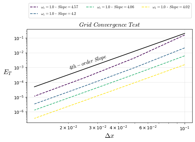
Fourth-Order Convergence
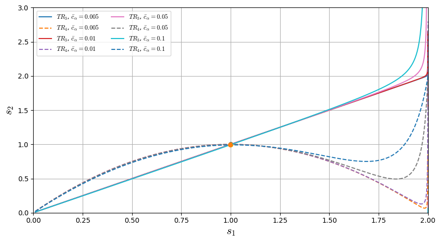
Making the term \(TR_{3}\) and \(TR_{4}\) equal zero and solving the equation, we have:
Plotting both solution for different values of \(\bar{c}_{\alpha}\):
Show code cell source
import numpy as np
import sympy as sp
import matplotlib.pyplot as plt
import matplotlib
matplotlib.rcParams['mathtext.fontset'] = 'cm'
# ---------------- Symbols ----------------
s1, s2, cbar = sp.symbols('s1 s2 cbar')
A = cbar**2

# ---------------- Eq 1: solve for s2 ----------------
s2_expr_1 = sp.solve(sp.Eq(A*s1*(s1*s2 - 3*s1 - 3*s2 + 6) + 2*(s1-2)*(s1-s2), 0), s2)[0]

# ---------------- Eq 2: s2(s1) (your big equation) ----------------
s2_expr_2 = (2*s1*(15*cbar**4*s1**2 - 18*cbar**4*s1
          - 3*cbar**2*s1**2 - 24*cbar**2*s1
          + 36*cbar**2 - 2*s1**2 + 8*s1 - 8)
) / (15*cbar**4*s1**3 - 24*cbar**4*s1**2
    + 3*cbar**2*s1**3 - 48*cbar**2*s1**2
    + 60*cbar**2*s1 + 4*s1 - 8)

# difference g(s1) = f1 - f2  (roots => intersections)
g_expr = sp.simplify(s2_expr_1 - s2_expr_2)

# lambdify for fast evaluation
f1 = sp.lambdify((s1, cbar), s2_expr_1, "numpy")
f2 = sp.lambdify((s1, cbar), s2_expr_2, "numpy")
g  = sp.lambdify((s1, cbar), g_expr,  "numpy")

# numeric root refinement (mpmath via sympy)
def refine_root(cb, x0):
    x = sp.nsolve(g_expr.subs(cbar, cb), s1, x0)
    return float(x)

def unique_sorted(xs, tol=1e-6):
    xs = sorted(xs)
    out = []
    for x in xs:
        if not out or abs(x - out[-1]) > tol:
            out.append(x)
    return out

# ---------------- Parameters ----------------
cbar_vals = [0.005, 0.01, 0.05, 0.1]
s1_min, s1_max = 0.01, 3.0
Nscan = 4000
s1_grid = np.linspace(s1_min, s1_max, Nscan)

# ---------------- Plot ----------------
plt.figure(figsize=(9, 5))

for cb in cbar_vals:
    y1 = f1(s1_grid, cb)
    y2 = f2(s1_grid, cb)
    yg = g(s1_grid, cb)

    # mask blow-ups / poles
    y1 = np.where(np.isfinite(y1) & (np.abs(y1) < 10), y1, np.nan)
    y2 = np.where(np.isfinite(y2) & (np.abs(y2) < 10), y2, np.nan)
    yg = np.where(np.isfinite(yg) & (np.abs(yg) < 1e6), yg, np.nan)

    # draw both curves
    plt.plot(s1_grid, y1, linestyle='-',  label=rf"$TR_{3}$, $\bar c_\alpha={cb}$")
    plt.plot(s1_grid, y2, linestyle='--', label=rf"$TR_{4}$, $\bar c_\alpha={cb}$")

    # --- find sign changes of g on the scan grid ---
    roots_guess = []
    for i in range(len(s1_grid) - 1):
        a, b = yg[i], yg[i+1]
        if np.isnan(a) or np.isnan(b):
            continue
        if a == 0.0:
            roots_guess.append(s1_grid[i])
        elif a * b < 0:  # sign change
            roots_guess.append(0.5 * (s1_grid[i] + s1_grid[i+1]))

    # refine guesses with nsolve
    roots = []
    for x0 in roots_guess:
        try:
            xr = refine_root(cb, x0)
            if s1_min <= xr <= s1_max:
                roots.append(xr)
        except Exception:
            pass

    roots = unique_sorted(roots, tol=1e-5)

    # compute s2 at intersection points and plot markers
    for xr in roots:
        yr = float(sp.N(s2_expr_1.subs({cbar: cb, s1: xr})))
        if np.isfinite(yr) and abs(yr) < 10:
            plt.plot([xr], [yr], marker='o', linestyle='None')

    if roots:
        print(f"cbar={cb}: intersections at s1 =", roots)

plt.xlabel(r"$s_1$",fontsize=16)
plt.ylabel(r"$s_2$",fontsize=16)
plt.xlim(0, 2)
plt.ylim(0, 3)
plt.grid(True)
plt.legend(ncol=2, fontsize=9)
plt.tight_layout()
plt.show()
cbar=0.005: intersections at s1 = [0.9999937477340344]
cbar=0.01: intersections at s1 = [0.9999749637281587]
cbar=0.05: intersections at s1 = [0.9993519974731944]
cbar=0.1: intersections at s1 = [0.9971142700951519]
Show code cell source
import warnings
warnings.filterwarnings("ignore")
import numpy as np
import matplotlib.pyplot as plt
import matplotlib
matplotlib.rcParams['mathtext.fontset'] = 'cm'
matplotlib.rcParams['mathtext.fontset'] = 'cm'
#--------------------------------------- Parameters (physical units) ------------------------------------------
A   = 1.0                         # Amplitude
phi = 0.0                         # Wave initial shift
k_w   = 1.0                       # Wave number
c   = 0.0125                         # wave speed
nu  = 0.066666666666666666*np.pi # Diffusive coefficient
m_waves = 1                       # Wave Period
L = m_waves * (2.0*np.pi / k_w)   # Domain Lentgh
t_end = 24.0                       # Final time
#--------------------------------------- Lattice-Properties-D1Q3 ----------------------------------------------
w = np.array([4.0/6.0, 1.0/6.0, 1.0/6.0],dtype="float64")
cx = np.array([0, 1, -1],dtype="int16")
cs=1.0/np.sqrt(3.0);
#--------------------------------- Initialization - Save Data Arrays -----------------------------------------------
cases=4
Nx0 = np.array([10, 20, 40, 80],dtype="int64")
r0 = 2**(0)*np.array([2.0**(1), 2.0**(2), 2.0**(3), 2.0**(4)],dtype="float64")
u_cases = np.empty(cases, dtype=object) # array field used to same data over time
for i in range(cases):
    u_cases[i] = np.zeros((Nx0[i]), dtype="float64")
for case in range(0,cases):
    #------------------------------------- Parameters (numerical units) -------------------------------------------
    Nx=Nx0[case]  # Numerical Length
    x  = np.linspace(0.0, L, Nx, endpoint=False,dtype="float64") # Numerical Domain
    dx = L / Nx # Grid size
    r = 1*r0[case] # dx/dt relation
    dt = dx/r
    ce = c/r
    nue = nu * dt / (dx*dx)
    tau1 = 0.5 + nue / cs**2
    om1=1.0/tau1
    om2=om1*(3.0*ce*ce*om1 - 6.0*ce*ce - 2.0*om1 +4.0)/(ce*ce*om1*om1 - 3.0*ce*ce*om1 - 2.0*om1 +4.0)
    tau2=1.0/om2
    nt = int(np.ceil(t_end / dt))
    print(f"dx={dx:.4e},\t dt={dt:.4e}\t nt={nt:d},\t tn={nt*dt:.2f}") # Print values for check
    print(f"c_lbm={ce:.3f},\t tau1={tau1:.4f},\t tau2={tau2:.4f}")
    print(f"s1={1.0/tau1:.4f},\t s2={1.0/tau2:.4f}")
    print(f"nt={nt:.3f}\t, nue={nue:.4f}")
    #--------------------------------- Initialization - LBM - Numerical Arrays -----------------------------------------
    u=np.zeros((Nx),dtype="float64")
    u = A * np.sin(k_w*(x+dx/2) + phi)
    mx=np.zeros((Nx),dtype="float64")
    mxx=np.zeros((Nx),dtype="float64")
    f=np.zeros((3,Nx),dtype="float64")
    feq=np.zeros((3,Nx),dtype="float64")
    fp=np.zeros((3,Nx),dtype="float64")
    for k in range(0,3):
        f[k,:]=w[k]*u[:]*(1.0 + cx[k]*ce/cs**2 + ce*ce*(cx[k]**2-cs**2)/(2.0*cs**4))
        fp[k,:]=w[k]*u[:]*(1.0 + cx[k]*ce/cs**2 + ce*ce*(cx[k]**2-cs**2)/(2.0*cs**4))
    #----------------------------------------- Init Loop --------------------------------------------------------
    for t in range(nt*10):
        #========================================= LBM - Solution =============================================
        #--------------------Collision----------------
        for k in range(0,3):
            feq[k,:]= w[k]*u[:]*(1.0 + cx[k]*ce/cs**2 + ce*ce*(cx[k]**2-cs**2)/(2.0*cs**4))
        mx = np.einsum('i,ix->x', cx, f-feq)
        mxx = np.einsum('i,ix->x', 3.0*cx*cx-2.0, f-feq)
        for k in range(0,3):
            fp[k,:]= feq[k,:] + w[k]*( (1.0-1.0/tau1)*cx[k]*mx[:]/cs**2 + (1.0-1.0/tau2)*(cx[k]**2-cs**2)*mxx[:]/(2.0*cs**2) )
        #-----------------streaming-------------------
        for k in range(0,3):
            f[k,:]=np.roll(fp[k,:], cx[k], axis=0)
    #----------------------------------------- Maind Loop --------------------------------------------------------
    for t in range(nt):
        #========================================= LBM - Solution =============================================
        #--------------------Collision----------------
        for k in range(0,3):
            feq[k,:]= w[k]*(u[:]+cx[k]*(ce*u[:])/cs**2 + u[:]*ce*ce*(cx[k]**2-cs**2)/(2.0*cs**4))
        mx = np.einsum('i,ix->x', cx, f-feq)
        mxx = np.einsum('i,ix->x', 3.0*cx*cx-2.0, f-feq)
        for k in range(0,3):
            # fp[k,:]= f[k,:] - w[k]*( cx[k]*mx[:]/(tau1*cs**2) + (cx[k]**2-cs**2)*mxx[:]/(2.0*cs**2*tau2) )
            fp[k,:]= feq[k,:] + w[k]*( (1.0-1.0/tau1)*cx[k]*mx[:]/cs**2 + (1.0-1.0/tau2)*(cx[k]**2-cs**2)*mxx[:]/(2.0*cs**2) )
        #-----------------streaming-------------------
        for k in range(0,3):
            f[k,:]=np.roll(fp[k,:], cx[k], axis=0)
        #----------------------Macro------------------
        # u[:]=f[0,:]+f[1,:]+f[2,:]
        u=np.einsum('ix->x', f)
    #---------------------save-field-cases--------------
    u_cases[case][:]=u[:]
Show code cell output
dx=6.2832e-01,	 dt=3.1416e-01	 nt=77,	 tn=24.19
c_lbm=0.006,	 tau1=1.0000,	 tau2=1.0000
s1=1.0000,	 s2=1.0000
nt=77.000	, nue=0.1667
dx=3.1416e-01,	 dt=7.8540e-02	 nt=306,	 tn=24.03
c_lbm=0.003,	 tau1=1.0000,	 tau2=1.0000
s1=1.0000,	 s2=1.0000
nt=306.000	, nue=0.1667
dx=1.5708e-01,	 dt=1.9635e-02	 nt=1223,	 tn=24.01
c_lbm=0.002,	 tau1=1.0000,	 tau2=1.0000
s1=1.0000,	 s2=1.0000
nt=1223.000	, nue=0.1667
dx=7.8540e-02,	 dt=4.9087e-03	 nt=4890,	 tn=24.00
c_lbm=0.001,	 tau1=1.0000,	 tau2=1.0000
s1=1.0000,	 s2=1.0000
nt=4890.000	, nue=0.1667
Show code cell source
#****************************************Data-Analysis*********************************************
# ---------------- exact solution ----------------
def u_exact(x, t, A, k_w, phi, c, nu):
# print(f"dx={dx:.4e},\t dt={dt:.4e}\t nt={nt:d},\t tn={nt*dt:.2f}")
return A * np.exp(-nu * k_w**2 * t) * np.sin(k_w * ((x+dx/2) - c*t) + phi)
u_ana = np.empty(cases, dtype=object) # array field used to same data over time
xl = np.empty(cases, dtype=object) # array field used to same data over time
for i in range(cases):
Nx=Nx0[i] # Numerical Length
x = np.linspace(0.0, L, Nx, endpoint=False,dtype="float64") # Numerical Domain
dx = L / Nx # Grid size
r = r0[i] # dx/dt relation
dt = dx/r
nt = int(np.ceil(t_end / dt))
xl[i] = np.linspace(0.0, L, Nx0[i], endpoint=False,dtype="float64")
u_ana[i] = np.zeros((Nx0[i]), dtype="float64")
u_ana[i] = u_exact(xl[i], nt*dt , A, k_w, phi, c, nu)
# -----------------Plot Results --------------------
plt.figure(figsize=(10,5))
colors = plt.cm.viridis(np.linspace(0, 1, cases))
for i in range(cases):
plt.plot(xl[i], u_cases[i], "s", color=colors[i], lw=1, label=f"LBM $Nx={Nx0[i]:.0f}$",fillstyle='none')
plt.plot(xl[i], u_ana[i], color=colors[i], lw=1, label=f"Exact $t={t_end:.2f}$")
plt.xlabel("$x$",fontsize=16)
plt.ylabel("$u(x,t)$",fontsize=16)
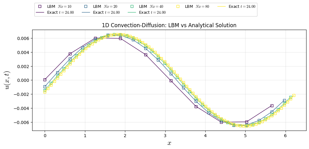
plt.title("1D Convection-Diffusion: LBM vs Analytical Solution")
plt.grid(True, alpha=0.3)
plt.legend(ncol=5,fontsize=9,loc="center left",bbox_to_anchor=(0.0, 1.2))
plt.tight_layout()
plt.show()
Show code cell source
Erro= np.zeros((cases), dtype="float64")
for i in range(cases):
    Erro[i]=np.sqrt(np.sum((u_cases[i]-u_ana[i])**2))/np.sqrt(np.sum((u_ana[i])**2))
    print(f'Erro{i}=',Erro[i])
TEp=np.polyfit(np.log(Nx0), np.log(Erro), 1)
print(TEp)
print(f'ltests[i] = np.array([{1/tau1:.2f},{c:.4f},{-TEp[0]:.2f},{Erro[0]},{Erro[1]},{Erro[2]},{Erro[3]}],dtype="float64")')
Show code cell output
Erro0= 0.0015336318570353604
Erro1= 9.266539911212256e-05
Erro2= 5.748285219599088e-06
Erro3= 3.5852375607247746e-07
[-4.01986148  2.76697863]
ltests[i] = np.array([1.00,0.0125,4.02,0.0015336318570353604,9.266539911212256e-05,5.748285219599088e-06,3.5852375607247746e-07],dtype="float64")
Show code cell source
#------------------ List of teste cases ---------------------------
ntests=4
ltests = np.empty(ntests, dtype=object) # list [omega, cs**2, a, erro1, erro2, erro3]
ltests[0] = np.array([1.00,1.00,4.57,0.15612287609561742,0.004397128432778937,0.00019967538064166106,1.135259052408131e-05],dtype="float64")
ltests[1] = np.array([1.00,0.50,4.20,0.02098923999495575,0.0009645322589991023,5.511609751733689e-05,3.3643885708974955e-06],dtype="float64")
ltests[2] = np.array([1.00,0.25,4.06,0.006086286711464546,0.0003438989164574731,2.0955010980109768e-05,1.3010601273425052e-06],dtype="float64")
ltests[3] = np.array([1.00,0.0125,4.02,0.0015336318570353604,9.266539911212256e-05,5.748285219599088e-06,3.5852375607247746e-07],dtype="float64")
Show code cell source
matplotlib.rcParams['mathtext.fontset'] = 'cm'
plt.figure(figsize=(7,4))
plt.title("$Grid$ $Convergence$ $Test$",fontsize=14)
colors = plt.cm.viridis(np.linspace(0, 1, ntests))
# plt.loglog(1/Nx0,ltests[0][3:],'r--',fillstyle='none', label=f'$\\omega={ltests[0][0]}$ - $Slope={ltests[0][2]}$')
for i in range(4):
    plt.loglog(1/Nx0,ltests[i][3:],'--',color=colors[i],fillstyle='none', label=f'$\\omega_{1}={ltests[i][0]}$ - $Slope={ltests[i][2]}$')

plt.loglog(1/Nx0,1.*2000.0/(Nx0**4),'k-',fillstyle='none')
plt.text(0.02, 0.0007, "$4th-order$ $Slope$", rotation=18,fontsize=12)
# plt.ylim(0,0.01)
plt.grid(True, alpha=0.3)
# plt.legend(loc=2,ncol=3,fontsize=8.5)
plt.legend(ncol=3,fontsize=9,loc="center left",bbox_to_anchor=(0.0, 1.2))
plt.ylabel('$E_{T}$',fontsize=16,rotation=0,horizontalalignment='right')
plt.xlabel('$\Delta x$',fontsize=16)
plt.show()