Diffusive Equation

The diffusive equation is described by

(18)\[ \partial_t \phi - \partial_{\alpha}\left( \nu \partial_{\alpha}\phi \right) = 0 \]

where \(\phi(\alpha,t)\) is a time and space dependent parameter and \(\nu\) is diffusive coeficient.

Numerical Discretization

../_images/mesh-1-diffusive.svg — Fig. 3 1D regular grid example for diffusive equation.

FDM Discretization

Discretizing the Eq. (18) through finite diference method, we have for forward time and central space (FTCS) discretizations:

\[ \partial_t \phi - \partial_{\alpha}\left( \nu \partial_{\alpha}\phi \right) = \frac{\phi(x,t + \Delta_{t}) - \phi(x,t) }{\Delta_{t}} - \nu\frac{ \phi(x - \Delta_{x},t) -2\phi(x,t) + \phi(x + \Delta_{x},t) }{\Delta_{x}^{2}} =0, \]

for \(\nu\) constant and isolating the term \(u(x,t + \Delta_{t})\), we can describe the \(\phi\) time evolution:

\[ \phi(x,t + \Delta_{t}) = \phi(x,t) + \frac{\nu\Delta_{t}}{\Delta_{x}^{2}} \left( \phi(x - \Delta_{x},t) -2\phi(x,t) + \phi(x + \Delta_{x},t) \right) . \]

Lattice Boltzmann Equation

Describing the problem through the BGK lattice Boltzmann equation (BGK-LB):

(19)\[ f_i( x_{\alpha} + c_{i,\alpha} \delta t, t+\delta t) = f_i(x_{\alpha}, t) -\left( \frac{ f_{i} - f_{i}^{eq} }{ \tau } \right), \]

where the equilibrium distribution function is defined by

\[ f^{eq}_{i} = w_{i}\phi(x_{\alpha}, t), \]

and the equilibrium moments are given by

(20)\[ \displaystyle\sum_{i=0} f_{i}^{eq}=\phi, \quad \quad \displaystyle\sum_{i}f_{i}^{eq} c_{i,\alpha} =0 \quad \quad \textrm{and} \quad \quad \displaystyle\sum_{i}f_{i}^{eq} c_{i,\alpha} c_{i,\beta} =c_{s}^{2} \phi \delta_{\alpha\beta}. \]

Through Chapman–Enskog analysis, it is demonstrated that the first-order non-equilibrium moment describes the pressure gradient and, consequently, the average velocity:

\[ m^{neq}_{\alpha} = \displaystyle\sum_{i} c_{i,\alpha}\left( f_i-f_i^{eq}\right) = -(c_{s}^{2} \tau \delta_{t})\partial_{\alpha}\phi \quad \quad \textrm{and} \quad\quad \tau = \displaystyle\frac{\nu}{c_{s}^{2} \delta_{t}} +\frac{1}{2}. \]

Lattice Direction Moments

\[\begin{split}\displaystyle \underbrace{\sum_{i=0} f_{i}^{eq} =\sum_{i=0} f_{i} }_{\textrm{Zero-Order Moment}} =\phi,\quad \quad \underbrace{\sum_{i=0} f_{i}^{eq}c_{i,x} }_{\textrm{x-First-Order Moment}} =0,\quad \quad \underbrace{\sum_{i=0} f_{i}^{eq}c_{i,y} }_{\textrm{y-First-Order Moment}} =0,\\ \quad \quad \underbrace{\sum_{i=0} f_{i}^{eq}c_{i,x}c_{i,x} }_{\textrm{xx-Second-Order Moment}} =\frac{\phi}{3},\quad \quad \underbrace{\sum_{i=0} f_{i}^{eq}c_{i,x}c_{i,y} }_{\textrm{xy-Second-Order Moment}} =0 \quad \quad and \quad \quad \underbrace{\sum_{i=0} f_{i}^{eq}c_{i,y}c_{i,y} }_{\textrm{yy-Second-Order Moment}} =\frac{\phi}{3}\end{split}\]

Chapmann-Enskog Analysis

Applying the Chapmann-Enskog procedure to LB equation, we expand the term \(f_{i}\left(\boldsymbol{x}+\boldsymbol{e}_i \Delta t, t+\Delta t\right)\) in a Taylor series to recover the derivative form of the equation, i.e.,

(21)\[ f_{i}\left( x_{\alpha} + c_{i,\alpha} \Delta t, t+\Delta t\right)- f_{i}( x_{\alpha}, t)=\displaystyle\sum_{j=1}^{\infty}\frac{\Delta t^{j}}{j!}D_{t}^{j}f_{i}= -\left( \frac{ f_{i} - f_{i}^{eq} }{ \tau } \right). \]

Rescaling the dimensionless form of the Eq. (21) in terms of the Knudsen number (\(Kn\)), we have

\[ \displaystyle \sum^{\infty}_{j=1} \frac{Kn^{(j-1)}}{j!} D_{t}^{j} f_{i} = - \frac{1}{Kn}\left( \frac{ f_{i} - f_{eq,i} }{ \tau } \right) \quad \quad \rightarrow \quad \quad \displaystyle \sum^{\infty}_{j=1} \frac{Kn^{(j)}}{j!} D_{t}^{j} f_{i} = - \frac{ f_{i} - f_{i}^{eq} }{ \tau }, \]

applying the asymptotic expansion in both the distribution function (\(f_{i}=f_{i}^{(0)}+Kn f_{i}^{(1)} + Kn^{2} f_{i}^{(2)}+\cdots\)) and time partial derivative (\(\partial_{t}=\partial_{t}^{(0)}+ Kn \partial_{t}^{(1)}+Kn^{2} \partial_{t}^{(2)}+\cdots\)), and separating the equation in orders up to the order \(Kn^{2}\):

(22)\[\begin{split} \begin{array}{ll} (Kn^{(0)}):& f_{i}^{(0)}= f_{i}^{eq},\\ (Kn^{(1)}):& \left( \partial_{t}^{(0)} + c_{i,\alpha}\partial_{\alpha} \right)f_{i}^{(0)}= - \displaystyle\frac{ f_{i}^{(1)} }{ \tau } , \\ (Kn^{(2)}):& \partial_{t}^{(1)} f_{i}^{(0)} + \left( \partial_{t}^{(0)} + c_{i,\alpha}\partial_{\alpha} \right)f_{i}^{(1)} + \displaystyle\frac{\left( \partial_{t}^{(0)} + c_{i,\alpha}\partial_{\alpha} \right)^{2} f_{i}^{(0)}}{2}= - \displaystyle\frac{ f_{i}^{(2)} }{ \tau },\\ \textrm{ou}\\ (Kn^{(2)}):& \partial_{t}^{(1)} f_{i}^{(0)} + \left( \partial_{t}^{(0)} + c_{i,\alpha}\partial_{\alpha} \right)\displaystyle\left(1 - \frac{1}{2\tau}\right) f_{i}^{(1)} = - \displaystyle\frac{ f_{i}^{(2)} }{ \tau } \quad\quad \rightarrow \quad\quad f_{i}^{(1)}\textrm{ Formulation} \\ \textrm{ou}\\ (Kn^{(2)}):& \partial_{t}^{(1)} f_{i}^{(0)} + \left( \partial_{t}^{(0)} + c_{i,\alpha}\partial_{\alpha} \right)^{2} \displaystyle\left(\frac{1}{2} - \tau\right) f_{i}^{(0)} = - \displaystyle\frac{ f_{i}^{(2)} }{ \tau } \quad\quad \rightarrow \quad\quad f_{i}^{(0)}\textrm{ Formulation}. \end{array} \end{split}\]

Zero-Order Moment Balance

To retrieve the balance equation, we sum the Eq. (22) for \(Kn^{(1)}\) and \(Kn^{(2)}\) over \(\sum_{i=0} \):

\[\begin{split} \begin{array}{l} (Kn^{(1)}): \displaystyle\sum_{i}\left( \partial_{t}^{(0)} + c_{i,\alpha}\partial_{\alpha} \right)f_{i}^{(0)}= \displaystyle\sum_{i} \left(- \displaystyle\frac{ f_{i}^{(1)} }{ \tau } \right),\\ (Kn^{(1)}): \partial_{t}^{(0)} \phi =0, \end{array} \end{split}\]

and

\[\begin{split} \begin{array}{l} (Kn^{(2)}): \displaystyle\sum_{i}\left( \partial_{t}^{(1)} f_{i}^{(0)} + \left( \partial_{t}^{(0)} + c_{i,\alpha}\partial_{\alpha} \right)^{2} \displaystyle\left( \frac{1}{2}-\tau\right) f_{i}^{(0)} \right) = \displaystyle\sum_{i}\left( - \displaystyle\frac{ f_{i}^{(2)} }{ \tau } \right), \\ (Kn^{(2)}): \partial_{t}^{(1)}\phi + \left( \displaystyle\frac{1}{2}-\tau\right) \partial_{\alpha}\partial_{\beta} \left(c_{s}^{2} \phi \delta_{\alpha\beta} \right) =0. \end{array} \end{split}\]

or

(23)\[\begin{split} \begin{array}{l} (Kn^{(2)}):& \displaystyle\sum_{i}\left[ \partial_{t}^{(1)} f_{i}^{(0)} + \left(1-\displaystyle\frac{1}{2\tau}\right)\left( \partial_{t}^{(0)} + c_{i,\alpha}\partial_{\alpha} \right) f_{i}^{(1)} \right]= \displaystyle\sum_{i}\left( - \displaystyle\frac{f_{i}^{(2)}}{\tau} \right), \nonumber \\ (Kn^{(2)}):& \partial_{t}^{(1)}\phi + \left(1-\displaystyle\frac{1}{2\tau}\right) m^{(1)}_{\alpha} = 0. \end{array} \end{split}\]

where \(m^{(1)}_{\alpha}\) is the first-order moment of \(f_{i}^{(1)}\) and \(\sum_{i=1}f_{i}^{(j)}=0\) for \(j\geq 1\) due to imposition of \(\phi\) conservation. To compute the moment \(m^{(1)}_{\alpha}\), we multiply Eq. (22) by \(c_{i,\alpha}\) and sum over all lattice directions:

(24)\[\begin{split} \begin{array}{l} (Kn^{(1)}): \displaystyle\sum_{i}c_{i,\alpha}\left( \partial_{t}^{(0)} + e_{\beta,i}\partial_{\beta} \right)f_{i}^{(0)}= \displaystyle\sum_{i} c_{i,\alpha} \left( -\frac{f_{i}^{(1)}}{\tau} \right),\\ (Kn^{(1)}): m^{(1)}_{\alpha} =-\tau \partial_{\beta}\left( c_{s}^{2} \phi \delta_{\alpha\beta} \right). \end{array} \end{split}\]

By substituting Eq. (24) into Eq. (23), we recover the Eq. (18), where \(\nu=c_{s}^{2}(\tau-1/2)\). In the regularized formulation of the lattice Boltzmann equation, the first-order correction is approximated as \(f_{i}^{(1)}\approx (f_{i}-f_{i}^{(0)})=f_{i}^{neq}\), where higher-order Knudsen moments are filtered out and the collision term is reformulated in terms of \(f_{i}^{neq}\).

Boundary Conditions

The boundary conditions for the lattices can be derived by solving a linear system of known moments.

D1Q2:	Boundaries	Layers
		West	East
	Unknown \(f_{i}\)	\(f_2=\phi_{e} - f_1\)	\(f_1=\phi_{w} - f_2\)

D1Q3:	Boundaries	Layers
		West	East
	Unknown \(f_{i}\)	\(f_2=\phi_{e} - f_1 - f_0\)	\(f_1=\phi_{w} - f_2 - f_0\)

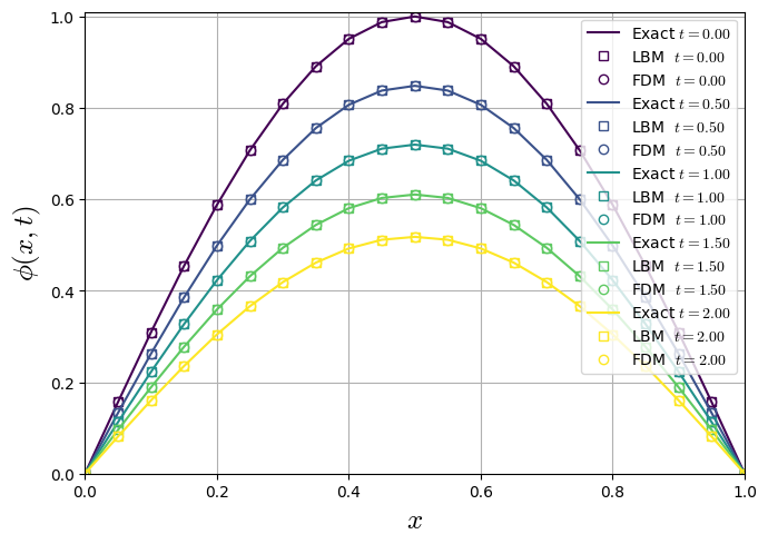
1st Benchmark: Single sine mode on a finite rod (Dirichlet)

PDE: \((\phi_t = \partial_{x}(\nu\partial_{x}\phi), (0<x<L,\ t>0)\)

BC: \((\phi(0,t)=\phi(L,t)=0)\)

IC: \(\phi(x,0)=\sin \left(\frac{\pi x}{L}\right)\)

Solution

\[ \phi(x,t)=\sin\left(\frac{\pi x}{L}\right) \exp \left(-\nu \frac{\pi^2}{L^2} t\right). \]

LBM D1Q3 Solution (\(\tau=1\))

Show code cell source Hide code cell source

import warnings
warnings.filterwarnings("ignore")
import numpy as np
import matplotlib.pyplot as plt
import matplotlib
matplotlib.rcParams['mathtext.fontset'] = 'cm'
#--------------------------------------- Parameters (physical units) ------------------------------------------
L = 1.0             # Length of the domain
nu = 0.1/3.0        # Diffusion coefficient
t_end = 2.0             # Total simulation time
#--------------------------------------- Lattice-Properties-D1Q3 ----------------------------------------------
cs=1.0/np.sqrt(3.0);
w = np.array([4.0/6.0, 1.0/6.0, 1.0/6.0],dtype="float64")
cx = np.array([0, 1, -1],dtype="int8")  
#------------------------------------- Parameters (numerical units) -------------------------------------------
Nx=21               # Domain Length
dx = L / (Nx-1)     # Spatial step size
c=1.0*2**(2)        # c=dx/dt
dt=dx/c             # Time step value
nt = int(t_end / dt)    # Time step number
nue=nu/(c*dx)       # Diffusion coefficient
tau=nue/cs**2+0.5   # Relaxation Time
print(f"dx={dx:.4e}\t dt={dt:.4e}\t nt={nt:d}") # Print values for check
print(f"nue={nue:.4f}\t tau={tau:.4f}")
#--------------------------------- Initialization - Numerical Arrays -----------------------------------------
T = np.zeros((Nx),dtype="float64")
x = np.linspace(0, Nx-1, Nx)
T = np.sin(np.pi * x / (Nx-1))
f = np.zeros((3,Nx),dtype="float64")
fp = np.zeros((3,Nx),dtype="float64")
for k in range(0,3):
    fp[k,:]=w[k]*T[:]
#--------------------------------- Initialization - Save Data Arrays -----------------------------------------
snaps=5 # number of states saved over time including 0 and t_end
T_snaps = np.empty(snaps, dtype=object) # array field used to same data over time
snaps_id = np.linspace(0, nt, snaps, dtype="int16") # timesteps to take the field
snap_index = {sid: i for i, sid in enumerate(snaps_id)}
for i in range(snaps):
    T_snaps[i] = np.zeros((Nx), dtype="float64")
T_snaps[0][:]=T[:]
#----------------------------------------- Maind Loop --------------------------------------------------------
for t in range(nt):
    #-----------------streaming-------------------
    for k in range(0,3):
        f[k,:]=np.roll(fp[k,:], cx[k], axis=0)
    #-----------------Boundaries-----------------------
    f[1,0]= 0.0 - f[0,0]-f[2,0]
    f[2,Nx-1]= 0.0 - f[0,Nx-1]-f[1,Nx-1]
    #----------------------Macro------------------
    T[:]=f[0,:]+f[1,:]+f[2,:]
    #---------------------save-snaps--------------
    if t+1 in snaps_id:
        i = snap_index[t+1]
        T_snaps[i][:]=T[:]
    #--------------------Collision----------------
    for k in range(0,3):
        fp[k,:]=f[k,:] - (f[k,:] - w[k]*T[:])/tau

FDM Solution

Show code cell source Hide code cell source

import warnings
warnings.filterwarnings("ignore")
import numpy as np
import matplotlib.pyplot as plt
import matplotlib
matplotlib.rcParams['mathtext.fontset'] = 'cm'
#--------------------------------------- Parameters (physical units) ------------------------------------------
L = 1.0            # Length of the domain
nu = 0.1/3.0           # Diffusion coefficient
t_end = 2.0             # Total simulation time
#------------------------------------- Parameters (numerical units) -------------------------------------------
Nx=21 #Square Domain Length
dx = L / (Nx-1)       # Spatial step size
c=1.0*2**(2)            # c=dx/dt
dt=dx/c             # Time step size
nt = int(t_end / dt)    # Time step number
print(f"dx={dx:.4e}\t dt={dt:.4e}\t nt={nt:d}") # Print values for check
print(f"nue={nue:.4f}\t tau={tau:.4f}")
#--------------------------------- Initialization - Numerical Arrays -----------------------------------------
Tf = np.zeros((Nx),dtype="float64")
x = np.linspace(0, Nx-1, Nx)
Tf = np.sin(np.pi * x / (Nx-1))
Tfp = np.zeros((Nx),dtype="float64")
#--------------------------------- Initialization - Save Data Arrays -----------------------------------------
snaps=5 # number of states saved over time including 0 and t_end
Tf_snaps = np.empty(snaps, dtype=object) # array field used to same data over time
snaps_id = np.linspace(0, nt, snaps, dtype="int16") # timesteps to take the field
snap_index = {sid: i for i, sid in enumerate(snaps_id)}
for i in range(snaps):
    Tf_snaps[i] = np.zeros((Nx), dtype="float64")
Tf_snaps[0][:]=Tf[:]
#----------------------------------------- Maind Loop --------------------------------------------------------
for t in range(nt):
    #--------------------Time iteration-----------
    Tfp[:]=Tf[:] + dt * nu * ( np.roll(Tf[:], 1, axis=0) -2.0*Tf[:] + np.roll(Tf[:], -1, axis=0) ) / dx**2
    Tf[:]=Tfp[:]
    Tf[0]= 0.0 
    Tf[Nx-1]= 0.0
    #---------------------save-snaps--------------
    if (t+1) in snaps_id:
        i = snap_index[t+1]
        Tf_snaps[i][:]=Tf[:]

Numerical and Analytical Comparisson

../_images/c5cc3526c8732aaa0be616770d2b1d08fd4eeb1a34ff574ad7def2c43353ee55.png

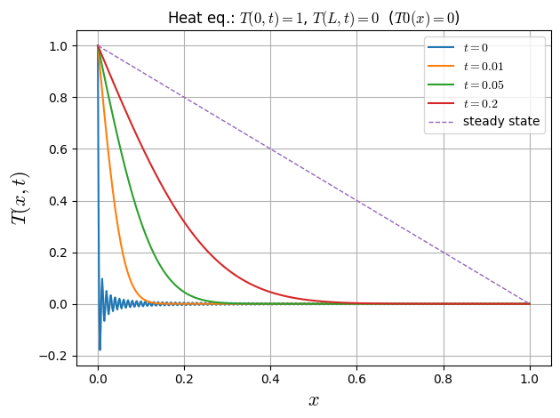
2nd Benchmark: Temperature ramp

Analyzing the accuracy of diffusive equation solver, we apply it to a one-dimensional analytical case. The geometry is described by a domain of length \(L\) initialized with a constant temperatura \(T(x,t=0)=0\). The boundary conditions are given \(T(x=0,t)=1\) and \(T(x=L,t)=0\).

Steady-State Analytical Solution

The analytical solution of this problem is given by:

\[ T(x,t\rightarrow \infty)= -\frac{x}{L} + 1. \]

Transient Analytical Solution

For the 1D heat equation \(\partial_t T=\nu\,\partial_{xx}T\) on \(0<x<L\) with

\[ T(0,t)=1,\qquad T(L,t)=0, \]

the steady state is \(T_{\text{ss}}(x)=1-\tfrac{x}{L}\). With \(u=T-T_{\text{ss}}\) (so \(u(0,t)=u(L,t)=0\)), the solution is

\[ T(x,t)=1-\frac{x}{L}+\sum_{n=1}^{\infty} B_n\,e^{-\nu (n\pi/L)^2 t}\,\sin\!\Big(\frac{n\pi x}{L}\Big), \quad B_n=\frac{2}{L}\int_0^L\!\Big[T_0(\xi)-\Big(1-\frac{\xi}{L}\Big)\Big]\sin\!\Big(\frac{n\pi \xi}{L}\Big)\,d\xi. \]

Special case \(T_0(x)=0\): \(B_n=-\dfrac{2}{n\pi}\), so

\[ T(x,t)=1-\frac{x}{L}-\frac{2}{\pi}\sum_{n=1}^{\infty}\frac{1}{n}\,e^{-\nu (n\pi/L)^2 t}\,\sin\!\Big(\frac{n\pi x}{L}\Big). \]

Here’s a ready-to-run Python snippet (with a single plot of \(T(x,t)\) vs \(x\) for multiple times):

Show code cell source Hide code cell source

import warnings
warnings.filterwarnings("ignore")
import numpy as np
import matplotlib.pyplot as plt
import matplotlib
matplotlib.rcParams['mathtext.fontset'] = 'cm'

# ---- Modes and series -------------------------------------------------------
def modes_dirichlet_dirichlet(L, N):
    n = np.arange(1, N+1)        # n = 1,2,...,N
    k = n * np.pi / L            # eigenvalues mu_n
    return n, k

def project_coeffs_dirichlet(T0_func, L, N, grid_pts=4000):
    """
    B_n = (2/L) ∫( T0(x) - T_ss(x) ) sin(nπx/L) dx, with T_ss = 1 - x/L.
    """
    x = np.linspace(0.0, L, grid_pts, endpoint=True)
    Tss = 1.0 - x / L
    u0 = T0_func(x) - Tss
    n, k = modes_dirichlet_dirichlet(L, N)          # (N,), (N,)
    S = np.sin(k[:, None] * x[None, :])             # (N, M)
    B = (2.0 / L) * np.trapz(u0[None, :] * S, x, axis=1)
    return B, n, k

def T_series_dirichlet(x, t, L, nu, B, k):
    """
    T(x,t) = T_ss(x) + sum_n B_n e^{-nu k_n^2 t} sin(k_n x), T_ss = 1 - x/L.
    """
    x = np.asarray(x)
    Tss = 1.0 - x / L
    coeff = B * np.exp(-nu * (k**2) * t)            # (N,)
    add = np.sum(coeff[:, None] * np.sin(k[:, None] * x[None, :]), axis=0)
    return Tss + add

# ---- Parameters -------------------------------------------------------------
L   = 1.0
nu  = 0.1
N   = 200
x   = np.linspace(0, L, 600)

# ---- Case A: initially cold rod T0(x)=0 (closed-form coefficients) ----------
n, k = modes_dirichlet_dirichlet(L, N)
B_cold = -2.0 / (n * np.pi)   # exact coefficients for T0 ≡ 0

times = [0.0, 0.01, 0.05, 0.2]

plt.figure()
for t in times:
    T_xt = T_series_dirichlet(x, t, L, nu, B_cold, k)
    plt.plot(x, T_xt, label=f"$t = {t:g}$")

# steady state
plt.plot(x, 1.0 - x/L, linestyle="--", linewidth=1, label="steady state")

plt.xlabel("$x$",fontsize=16)
plt.ylabel("$T(x,t)$",fontsize=16)
plt.title("Heat eq.: $T(0,t)=1$, $T(L,t)=0$  ($T0(x)=0$)")
plt.legend()
plt.grid(True)
plt.tight_layout()
plt.show()

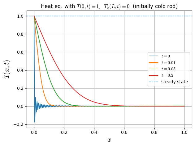
../_images/2403470fec7d4e060ad997d120a119634f7db0e84ddd220de8334dace53cc433.png

3rd Benchmark: Temperature Ramp with Adiabatic Boundary

Assuming the forward heat equation in 1D with constant diffusivity \(\nu>0\),

\[ \partial_t T=\nu\,\partial_{xx}T,\qquad 0<x<L,\ t>0, \]

and the mixed boundary conditions

\[ T(0,t)=1,\qquad \partial_x T(L,t)=0, \]

the steady state is \(T_{\mathrm{ss}}(x)=1\).

Let \(u(x,t)=T(x,t)-1\). Then \(u\) solves

\[ \partial_t u=\nu\,\partial_{xx}u,\quad u(0,t)=0,\quad \partial_x u(L,t)=0,\quad u(x,0)=u_0(x):=T_0(x)-1. \]

Separation of variables with eigenfunctions satisfying \(X(0)=0,\ X'(L)=0\) gives

\[ X_n(x)=\sin(\mu_n x),\qquad \mu_n=\frac{(n+\tfrac12)\pi}{L},\quad n=0,1,2,\dots \]

Hence the solution is the sine‐series

\[ \boxed{\ T(x,t)=1+\sum_{n=0}^{\infty} A_n\,e^{-\nu\,\mu_n^{2}\,t}\,\sin(\mu_n x),\qquad \mu_n=\frac{(n+\tfrac12)\pi}{L},\ } \]

with coefficients (using \(\int_0^L \sin(\mu_m x)\sin(\mu_n x)\,dx=\tfrac{L}{2}\delta_{mn}\))

\[ \boxed{\ A_n=\frac{2}{L}\int_0^L \big[T_0(\xi)-1\big]\sin(\mu_n \xi)\,d\xi.\ } \]

Common special case (initially cold rod): if \(T_0(x)=0\), then \(u_0(x)=-1\) and

\[ A_n=\frac{2}{L}\int_0^L (-1)\sin(\mu_n \xi)\,d\xi=-\frac{2}{L\mu_n}, \]

so

\[ \boxed{\ T(x,t)=1-\sum_{n=0}^\infty \frac{2}{L\mu_n}\,e^{-\nu\,\mu_n^{2}\,t}\,\sin(\mu_n x),\qquad \mu_n=\frac{(n+\tfrac12)\pi}{L}.\ } \]

Note: if you literally use your original sign \(\partial_t T+\nu T_{xx}=0\) (the backward heat equation), the time-dependent problem is ill-posed forward in \(t\). For a physically meaningful diffusion process, use \(\partial_t T=\nu T_{xx}\).

../_images/9d36f688a2acd06f0e0f919f38d1395b30db333af6d6dda4984df3da6b6439aa.png